My basic nonlinear processing of an RGB image from start to finish.
In the following article, we will see what is my basic workflow, to process a three channel color image ( RGB ) , obtained with an OSC camera.
In this particular case it is a dedicated and cooled camera for astrophotography, with an APS sensor ( Sony IMX-571 ), similar to that of a conventional DSLR, although with a higher quantum efficiency (QE), and a deeper dynamic range (16 bits) than most conventional DSLRs (12/14 bits), whose only filter is a protective glass that cuts UV and IR.
The shots were taken in November 2024 from Cinctorres , a village in the interior of Castellón that has a relatively dark sky ( Bortle 3 ), being B1 the darkest, equivalent to being in the middle of the ocean far from the coast and B9 the brightest, equivalent to looking at the sky from the center of a big city like Madrid or Barcelona.
If you want to consult the map of light pollution, click on this LINK
There are 13 hours of total integration in individual shots (subframes) of 300″ at -10º and gain 101, with a wide field telescope, the Askar FMA 180 Pro , which together with the pixel size of the camera (3.76µ), gives me a resolution of 4.31″ of arc per pixel and a field of 7.47º x 4.99º, a very wide field.
If you want to know the resolution of your optical assembly (camera/tube), you can click on this LINK.
Having said that, let’s go to the heart of the matter, remember that we have already finished the whole linear process, you can see it in this ARTICLE, now it’s time to illuminate and contrast, also known by the acronym DDP or Digital Development Process.
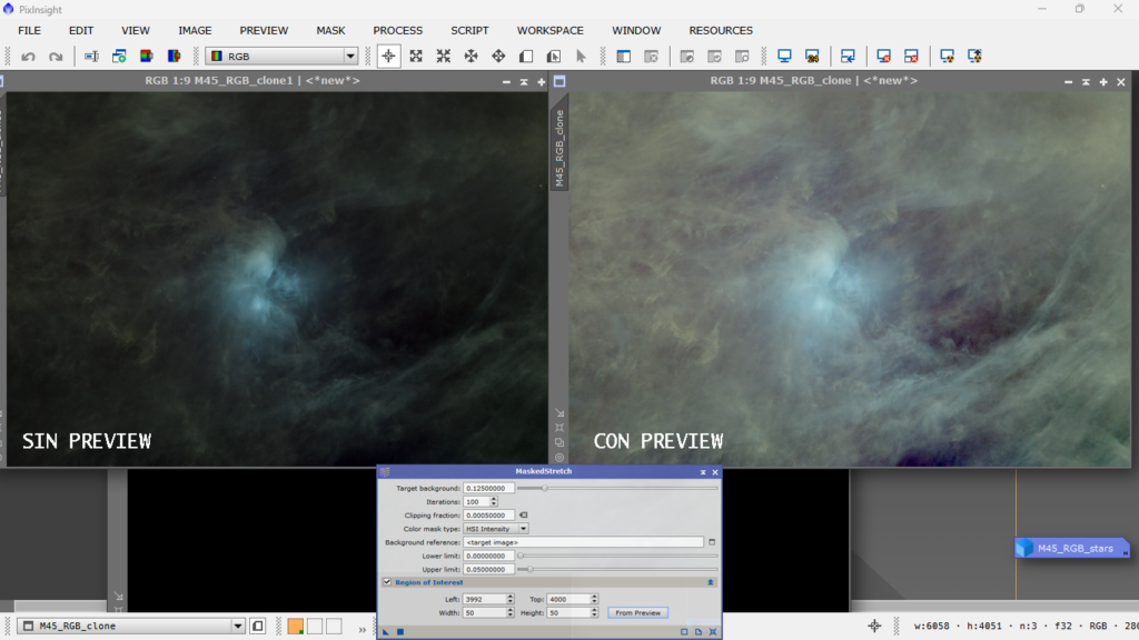
Before getting into the subject, I would like to make a brief comment about the Masked Stretch configuration. If we define a background preview as little affected as possible by foreground objects such as nebulae, stars, etc., we will obtain a more intense stretch. I am comparing this with background preview and without preview, i.e. using the whole image as evaluation model. I prefer it without preview, so that I can stretch it little by little afterwards and preserve details and colors better, but well, it’s all a matter of taste.
PS: To define the background sample, I used SetiAstro’s FindBackground script.
Here is the comparison:
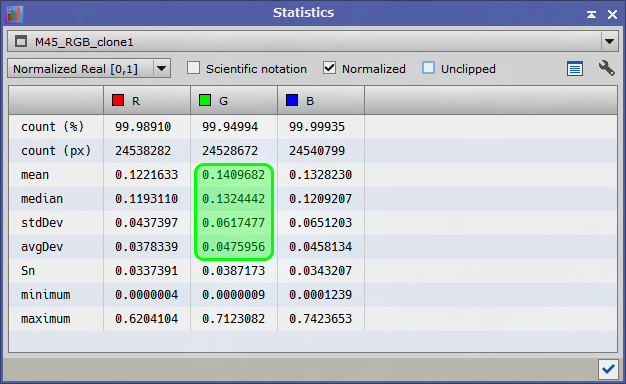
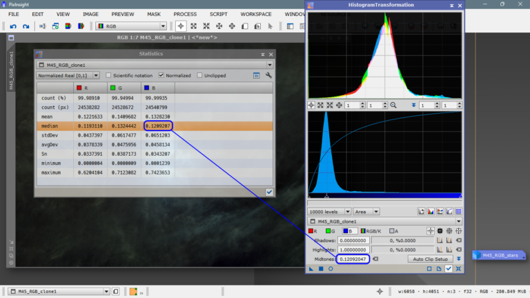
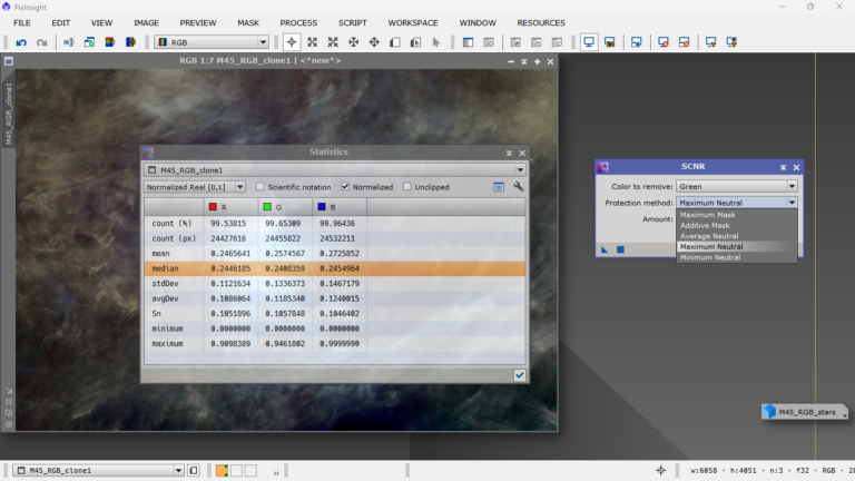
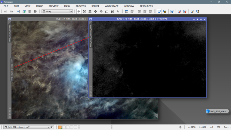
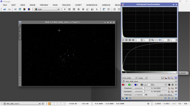
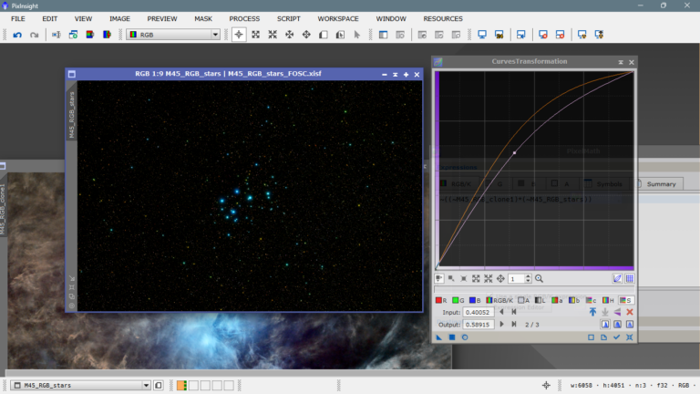
At this point, I start by checking the histogram, but above all I look at the statistics, if I take into account that it is a broadband image, without any kind of filter, except the IR/UV that the camera has in the protective window, the green color cannot dominate the scene, so I inspect the photo, first visually, and I already see a greenish tone, I read the statistics and see that the illumination of the green channel is higher than that of the blue, and much higher than that of the red, in principle nothing would happen because our sensor is RGGB, ie, the information that has fallen in each pixel, the green channel has been doubly protagonist independently of the intensity and composition of this object, which as we all know is a nebula of reflection of the light of young and very hot stars that as we all know, are of spectral type B, ergo the light reflected in the surrounding dust should have at most, a bluish dominant and not greenish, this excess of green must be balanced either by subtracting chromatic noise with SCNR, or by equalizing the average values of each channel manually, in the old school style.
I have to say that I apply both methods combined, first I equalize the illumination of the three channels and then I remove chromatic noise with SCNR, if it is still very evident, I use the Medium Neutral function, and if it is more contained I use Maximum Neutral.
Let’s see the statistics and how the green channel is brighter:
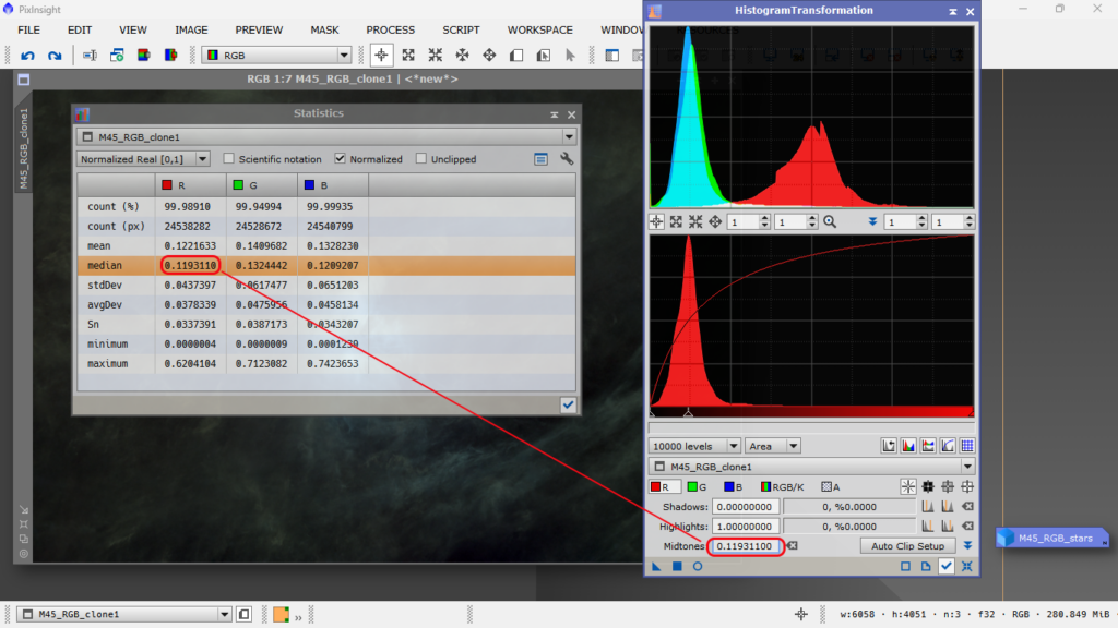
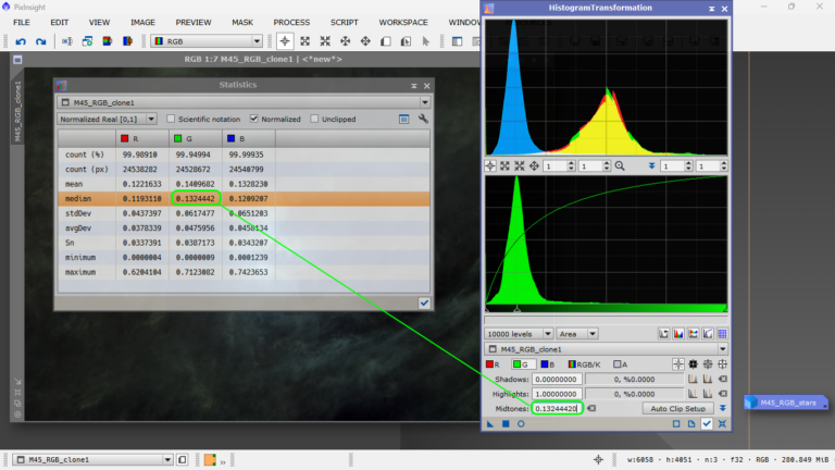
What I do now is to equalize the illumination values of the three channels, inserting the median value of each channel, in the histogram halftone box, channel by channel, and once done, lower the RGB channel to the same height as the bell below, the one that has not moved, so what I get is to equalize the color and get rid of any dominant intensity. Obviously, I will have to correct if there is any green area left, remember that except for comets and planetary nebulae, there is no object emitting in the visible that is green.
Let’s go there, I copy the median value of the red channel and insert it as a halftone value of the same channel, I also do this in the green channel and in the blue channel, every time I paste a value, I hit enter to apply it.
Red channel:
Green channel:
Blue channel:
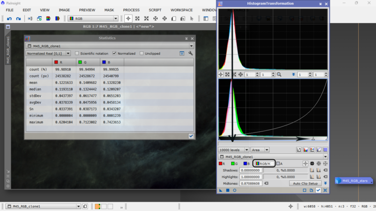
The combined channel (RGB), we equalize it in intensity with the previous state, moving the halftone arrow to the right, until the new bell coincides with the previous bell, the one below.
We apply and take a look at the image, in case we still detect green dominant, at first glance it seems that no….but….
We cannot rely only on our eyesight, we must check the statistics to be more accurate and objective.
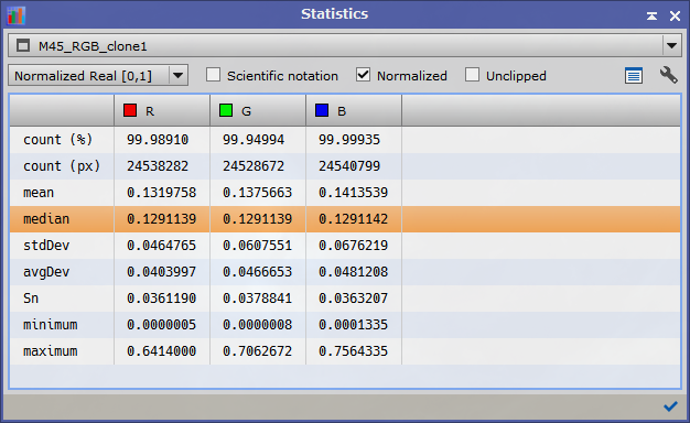
We see that our eyes are still in shape hehehe, we have a wide band image, well balanced, no green dominants or any other color, we see that the image of M 45 is what we expect from it, blue nebulosity the closer to the stars and a more reddish tone the farther we move away, well.
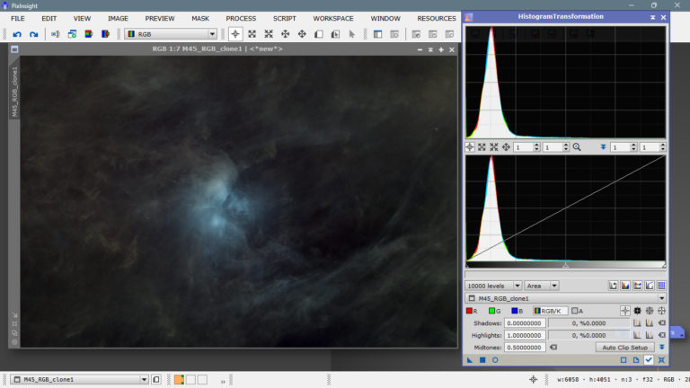
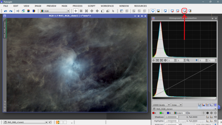
The next step is to brighten the panorama in a weighted way, I really like to do it with the nuclear radiation icon hehehe, of the two there are, the one on the left makes a smoother screen transfer than the one on the right, what I do is click on that icon, open STF and transfer those settings to the histogram to be applied “for real”, by throwing the triangle in the lower left corner, over the lower part of the histogram window.
I click on the nuclear radiation icon:
Now I open STF and transfer those settings to the histogram:
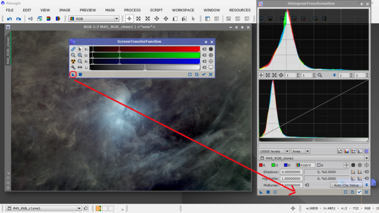
With the track view activated, I reset it so as not to get a scare later.

And I apply the histogram transformation
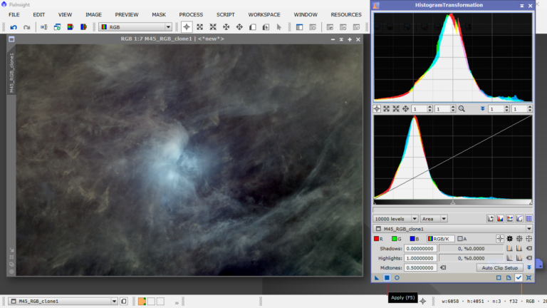
Now I have a well stretched image, not flat at all, with enough contrast, ready to continue with the processing.
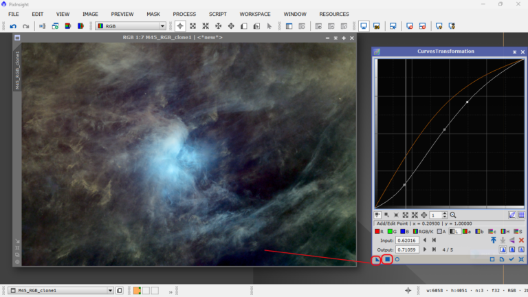
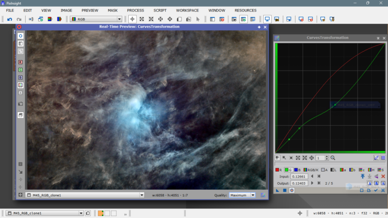
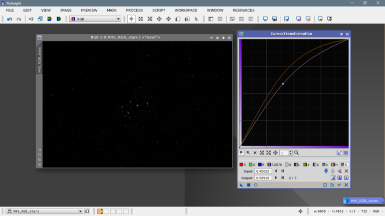
Next I am going to deal with the color, I personally like strong images, with just enough contrast but the color of each element is well seen, so I go to the curves and play with the balance Luminance vs Chrominance, L channel vs C channel.
I start by going up the chrominance curve and see how it affects the different colors in the image.
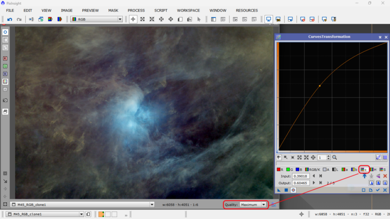
I like it, I see that green is starting to emerge in areas where the color is supposed to be more neutral, I will keep this in mind in the next step. Now WITHOUT APPLYING, I will play with the Luminance curve to try to give more contrast, that is to say, to darken areas that are too bright so that there is a transition between the different parts of the photo, so that it doesn’t look flat. Now we can apply the transformation, we have an image with a good contrast and a good color, keep in mind that the luminance and chrominance are antagonistic, ie, if you raise one, the other goes down and vice versa.
Now we apply by clicking on the square or by throwing the triangle on the image:
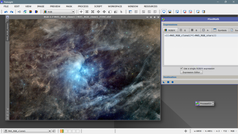
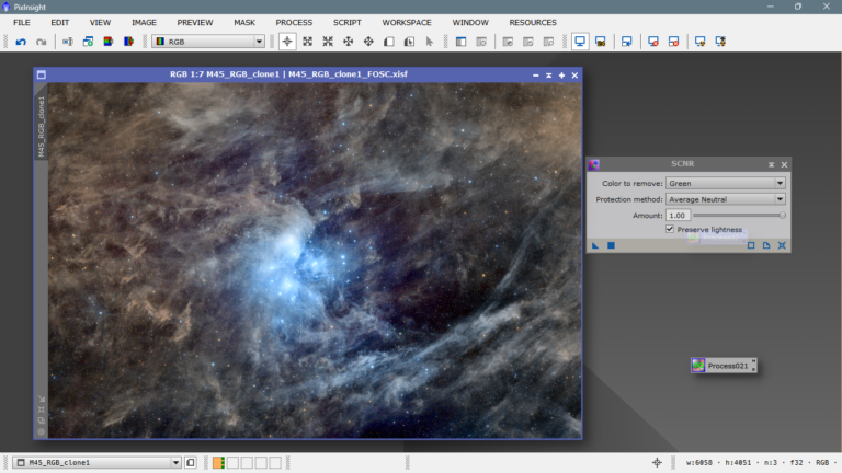
The color and contrast are very good except for the green that swarms around, as I said before I will try between Average Neutral and Maximum Neutral, here what happens is that if we remove a lot of green we will give a pinkish tint to areas of red where the green contributes to give a more yellowish aspect, more of galactic dust, then we must be careful and test until we find the key.
After making several tests and looking a lot at the statistics, I have decided for the Maximum Neutral method of SCNR, even though there is no documentation, the experience I have with SCNR leads me to think that the mask to protect the color, makes it using the maximum values of the desired channel, instead, with Average Neutral builds the mask based on an arithmetic mean of values, so one protects more than another and removes more color one than another, I have stayed with Maximum, because I have found more balanced statistics:
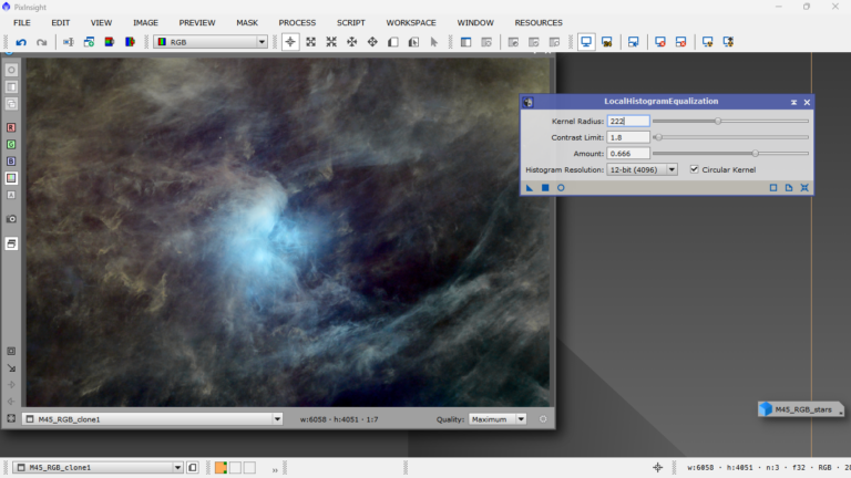
Then, the next step is to get more definition in the structures, what we call wavefronts, that is, where one structure ends and another begins, we can do two things, increase the local contrast, ie change the light in a very localized way, to structures of different sizes and/or deconvolute these structures, be careful with the deconvolution, because the image being so stretched, can cause artifacts very easily, so you have to be gentle and take previews, test and be patient.
I liked these settings, with the real time window is enough, here it is not necessary to make previews, but be careful with this tool, it is very greedy and when you realize you have spent four villages hehe, in another article I will explain how LocalHistogramEqualization works, it is very simple, but we will see it later, for now the recommendation is not to be aggressive and set the histogram resolution the higher the better, more precision, yes, the process will be much slower, but it is worth it.
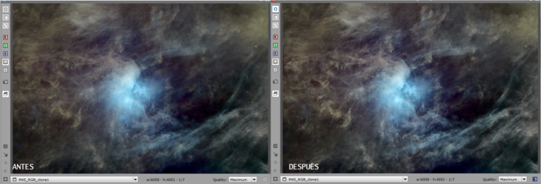
before/after
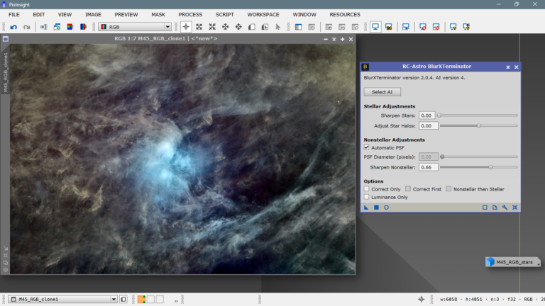
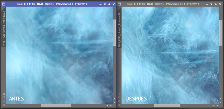
Well, now it’s time for the “sharpening” of the structures, for this I will use BlurXterminator in “Sharpen Nonstellar” mode only, I will leave all the other parameters inactive and at zero and I will focus exclusively on this one, being very careful not to create artifacts, because with this tool it is very easy to overdo it. After several previews of different areas of the sky, I have decided to leave it at 66% of aggressiveness, getting a good result and no trace of artifacts.
The change is remarkable, and although it introduces large-scale noise, it is worth it:
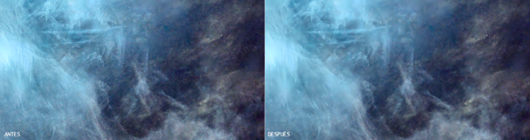
To solve the issue of large-scale noise, or noise produced by the processing itself, I like to resort to my old GreycStoration that works wonders in very bright images, I applied the default parameters and the result is highly satisfactory.

zoom
Now let’s try to give our color the last finishing touch, before adding the stars. I still find that greenish color that can be seen in the surrounding structures, which is actually galactic dust and we don’t know for sure which color is the “real” one, I put a lot of emphasis on that term, anyway, I let myself be guided by my prejudices and my influences of seeing photos for many years and I will leave them with a color that fits my standards, I reiterate that at this point, the processing becomes something very personal and as long as you don’t paint the Pleiades in fuchsia or yellow, all these nuances are totally legitimate and very personal, let the record show.
Well, what I’m going to do is to alter the color composition of certain structures to suit what I want, those surrounding structures so yellow, I would like to see them more brownish, then I imagine they are red structures that have too much green (red + green = yellow), well, I will create a mask with the luminance of the red plus the luminance of the green and so I will have a mask for the yellow color, it can be done manually, but you can get them faster but not as perfect as the manual ones, with the native script Color Mask.
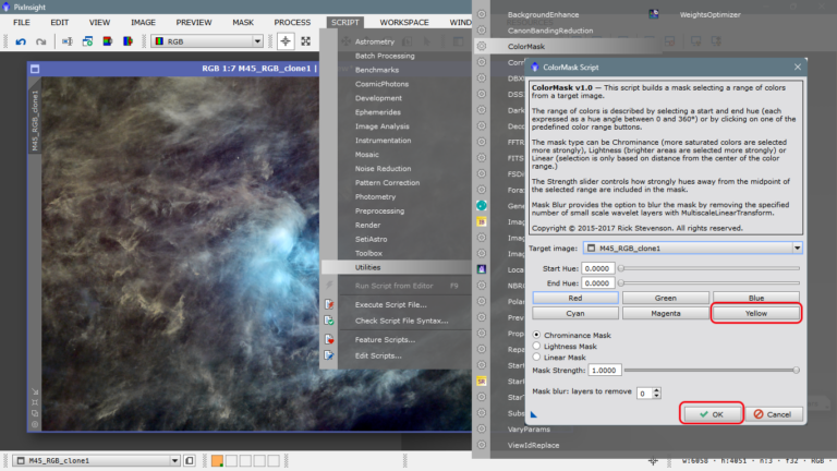
We make the yellow mask and apply it on the image by launching the tab on the side bar of the window
It is assumed that now we have everything protected except the yellow or yellowish structures, that is, they are structures that have part red and part green, so they are yellow, what we will do, if what we want is to change the color to a more brownish one, is to lower the green or raise the red and thus change the hue of these structures, let’s do it.
I keep these settings and apply them on the image.
The yellowish structures are browner and the greener ones are more neutral. Let’s remember to remove the mask.
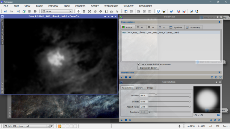
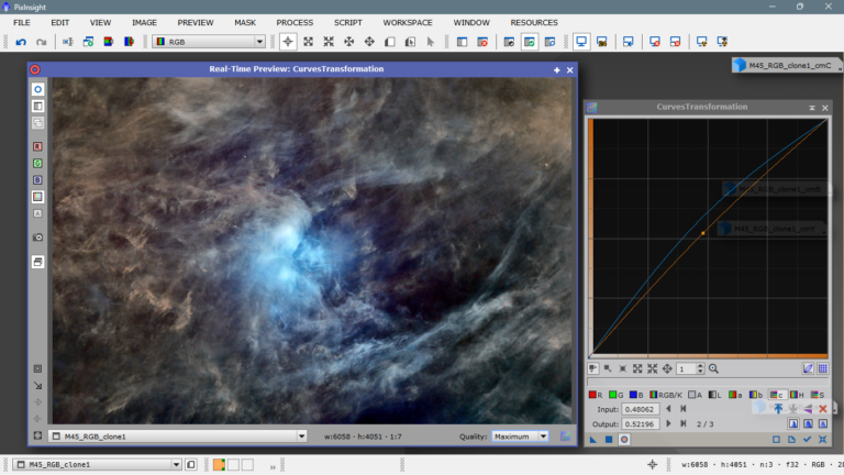
Let’s go for the blues, I would like the blue surrounding the Pleiades, to be more extensive, more solid and with better contrast, for this I have made two masks, one with the cyan evident in the image, and another with the blue, I have mixed them in Pixelmath making a sum of maximums to have the most illuminated of each of them, and then I have blurred them in Convolution to not create artifacts around the mask.
Then I went to the curves and applied this instance:
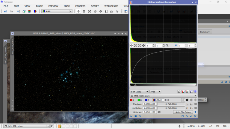
At this point, it is time to stretch and process the stars, remember that we had them separated before the first stretching, they are only deconvoluted, but remain linear, without stretching. We are going to stretch them using the histogram, set to 8 bits and raise the arrow of the midtones to where the data bell starts (or ends, depending on how you look at it), I always do it this way more than anything to have a reference and always do the same, I have done it so many times and I know it works, that I resist to change the method.
We will not reset the histogram, since if the stars seem to be a little stretched, it will be enough to reapply it as it is, in the same way.
Now we will go to the curves and saturate them to show the color better.
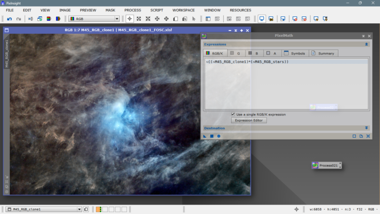
And finally we will apply a Pixel Math formula, remember that we can apply different formulas to obtain the same or similar result, what they all have in common is that the background of the photo of the stars is not added to the photo of the nebulae, although we can do it by a rescaled sum, but the photo would be much darker by adding the values of the shadows of the photo of the stars only. I use a very common formula, I have it saved in a process icon and when I go to add the stars I don’t have to write it every time, it is very easy to save, just drag the triangle of Pixel Math (or any other tool) to the bottom of the desktop, and it becomes an icon that we can save and rename, we can even embed a small documentation in case we forget what we have saved it for hehe. Well, the formula I use is this : ~((~)*(~)) and it is written like this:
~((~picture with stars)*(~picture without stars))
We can also use this formula, simpler and just as effective: Max(,)
Max(image with stars,image without stars) where only the maximum values of each image are mixed.
When applying we see that we have fallen short, so nothing, we return to the histogram that we have NOT reset, and we give them another stretch.
We go back to Curves Transform, and with the same parameters as before, we return to saturate, remember that when we stretch an image and it gains light, it loses color, so we must recover the lost color.
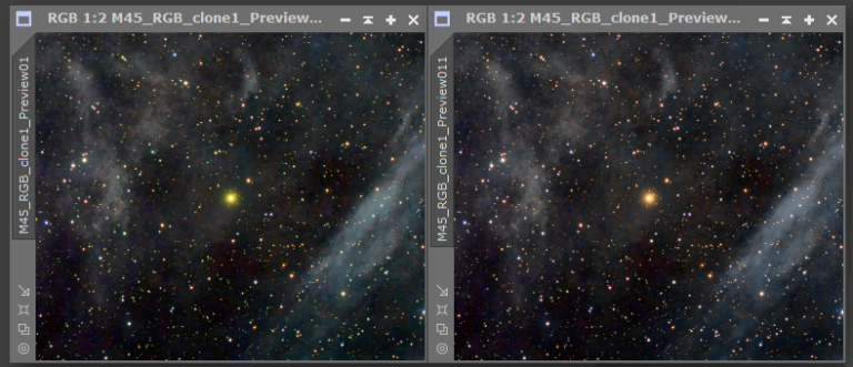
Now we go back to the nebulae-only image, undo to remove the stars and apply the PixelMath instance again.I like them as they are, but if you like them with more presence, it will be enough to launch the Pixel Math instance, as many times as we believe necessary until we reach the desired aspect, for example, after launching PixelMath four times (compare with the one above):
Now we only need the final touch, which in my opinion would be to pass SCNR to see if there is any green left, both in the nebulae and in the stars, especially in the latter, notice how the nebula becomes more blue, and especially the star on the right that looks yellow, becomes more orange.
zoom
And we would already have the finished image, now it would depend on the taste of each one if to remove more noise, if to saturate more the colors, to sign it, etc etc etc.
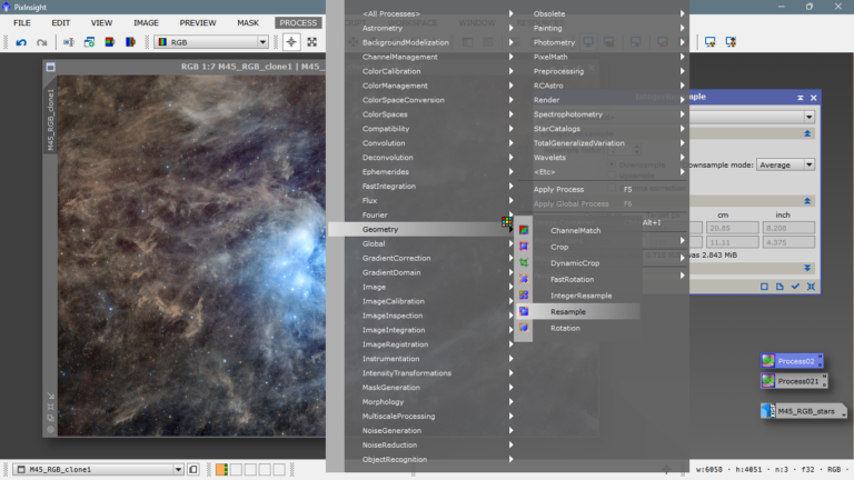
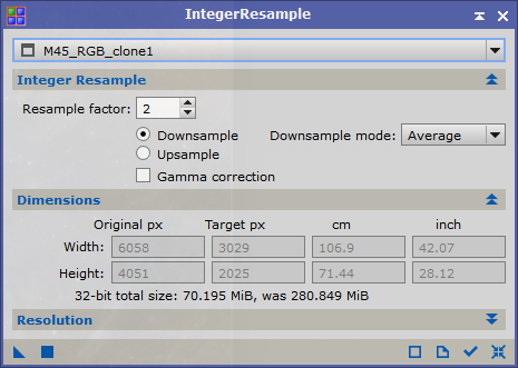
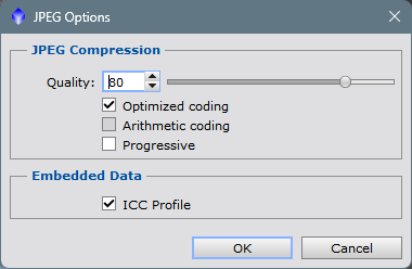
I usually save it in .XISF and .jpeg at half size to put it on the internet, I do it with Geometry/Integer Resample/Downsample(2) and save it in jpeg at 100% quality, if I want it to occupy less space, then I lower the quality to 80%, etc.
If you want to process it yourselves, here you have the master, click on this LINK, if you want to share your processing and what you would improve, or what you would not do, or if you would do it differently, so we can learn from each other.
And this tuto is over, greetings, I hope you liked it and that you find it useful.
See you next time!