My logical order of work and its logic.
When we start to process a photo in PixInsight, the data are linear, that is, we have quantity but almost no intensity, so we see the photo black, or simply with four white dots corresponding to very bright stars. Processing data in LINEAR, means that we have to prepare the image, clean it of noise, refocus it to combat the “blur” effect of the atmosphere, add astrometric data if necessary, calibrate the color, fix the stars, correct the gradients caused by light pollution, etc., all without altering the intensity, because if we did, the data would no longer be those we have captured, but those we have transformed, and how to do that will come later, in the next article.
In this article, I will explain the way and the order in which I do it, how I do it and why I do first one thing and then another and not the other way around.
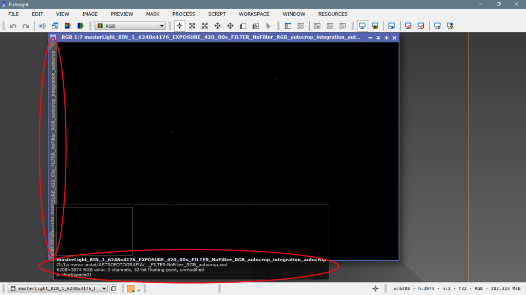
When opening the image, the first thing we have to do is to change the name of the photo, since they come out of the WBPP (the calibration tool) with a very long name and for convenience it is better that the tab is short, since as we will see later, the PixInsight tabs are dynamic and you can do many things with them, so it is better that the name is short. Notice now how long it is:
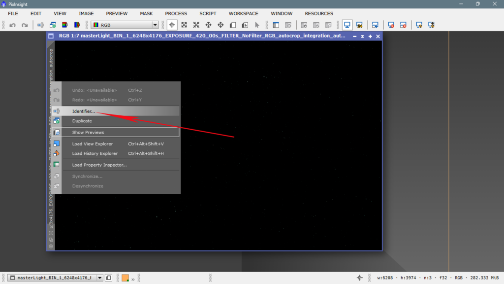
Simply place the pointer over the left tab, right-click and change the name by clicking on Identifier.
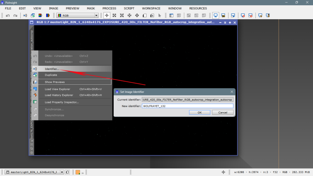
As it is a photo of the Wolf-Rayet 134, I give it that name.
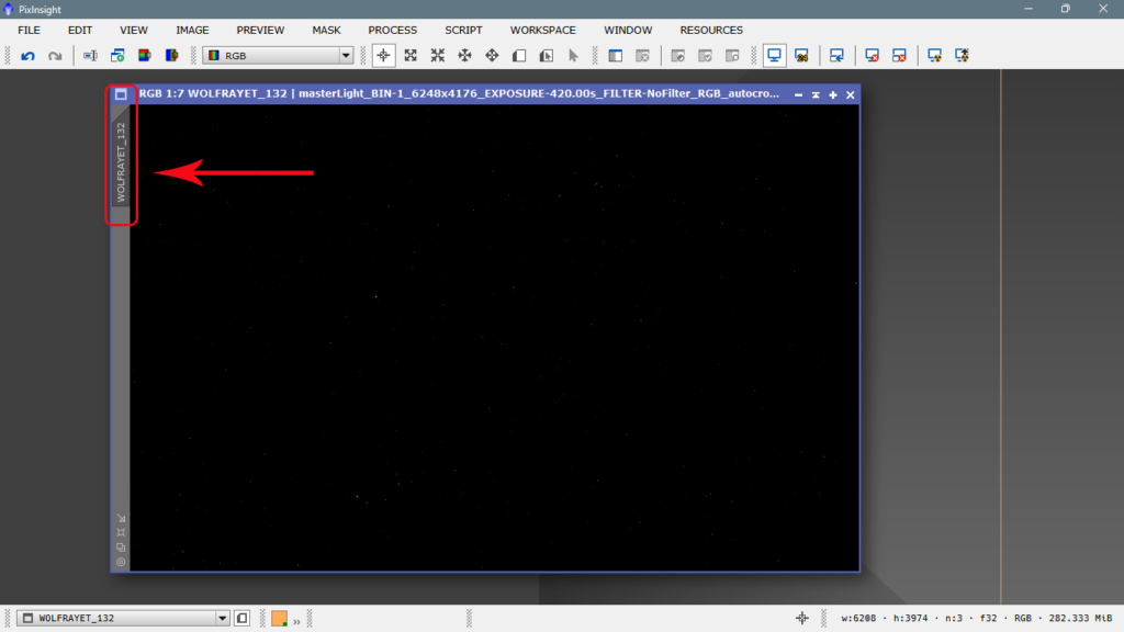
Now the tab is shorter and easier to handle.
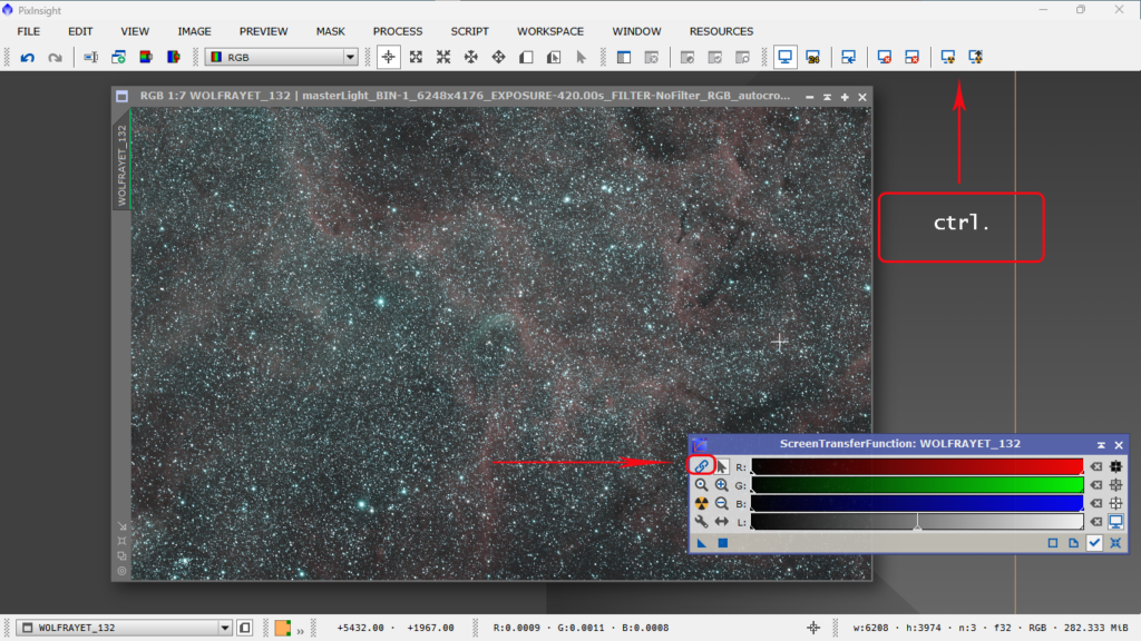
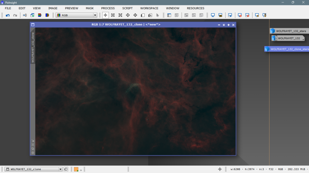
The next step is to illuminate the image in a virtual way, that is, it is an image that simply shows what is there but does not apply any kind of real striatum (intensity) to the image, it is like a preview. We do it from Screen Transfer Function or from the upper toolbar, using the radioactivity icons.
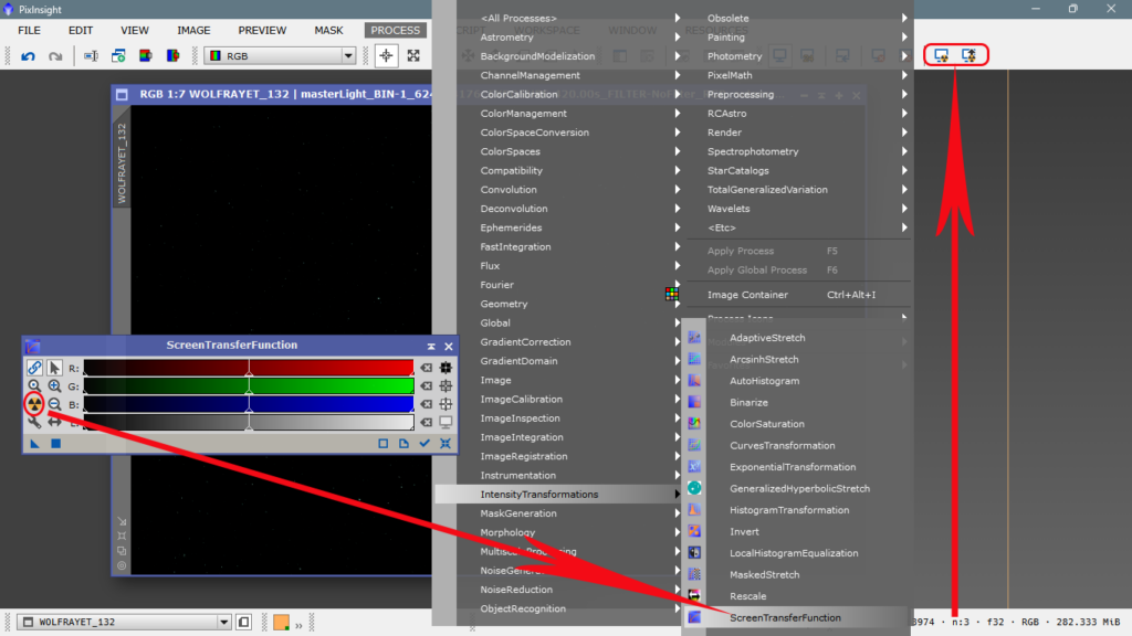
Now we have the image falsely stretched to be able to see what is there, IMPORTANT to unlink the channels from each other, from the link symbol if we use STF, or pressing ctrl. if we use the upper icons, otherwise we will see everything green.
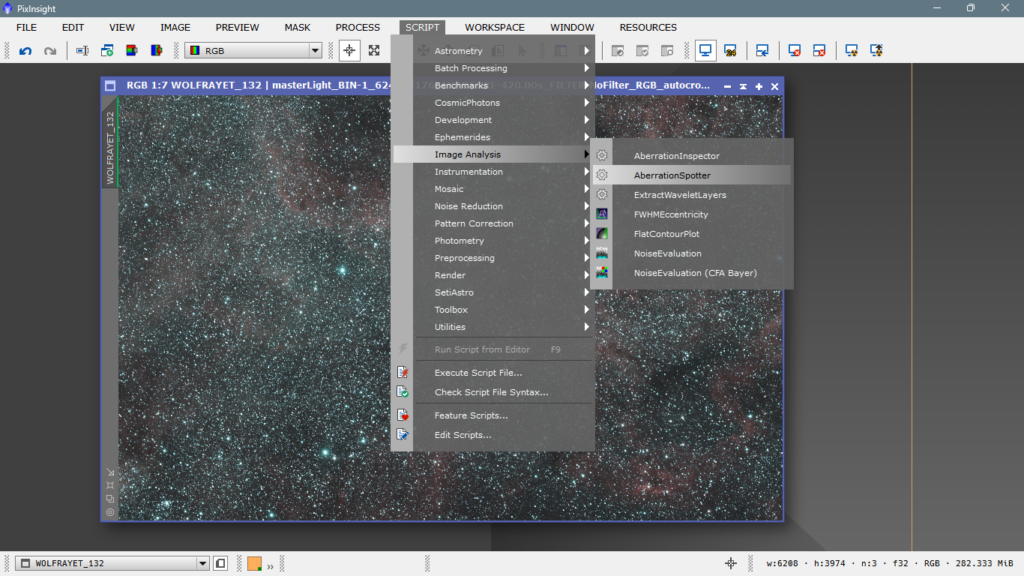
The first thing we have to do is to inspect how the stars have turned out, especially those in the corners, which are the most prone to suffer distortions due to geometric aberration. To do this we will use the native script AberrationSpotter, from SCRIPT/Image Analisys/AberrationSpotter.

The script console will be displayed, where we can choose the size of the squares and whether or not we want to see the central stars.
Once configured to your liking, click on OK and you will obtain the following image that you will also have to pass it through STF to be able to see it.
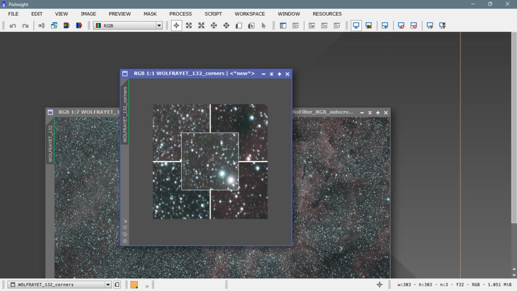
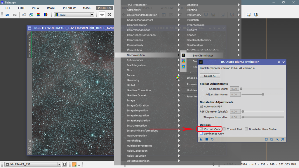
It is evident that the stars are very improvable, they have geometric aberration, guiding defects, a little bit of astigmatism and also a little bit of chromatic aberration, the logical step is to correct these defects, and to do this we will use the deconvolution tool BlurXterminator, for the moment we will select the option “Correct Only” to correct only the shape of the stars that are not quite round.
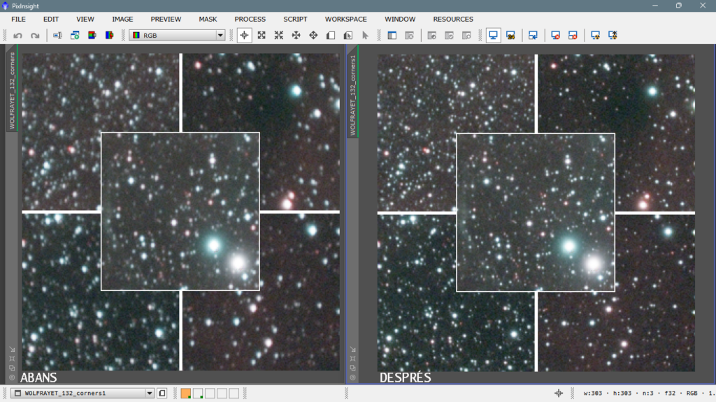
After application, we can see that it has worked like a charm, the shape is now quite round and much better than before.
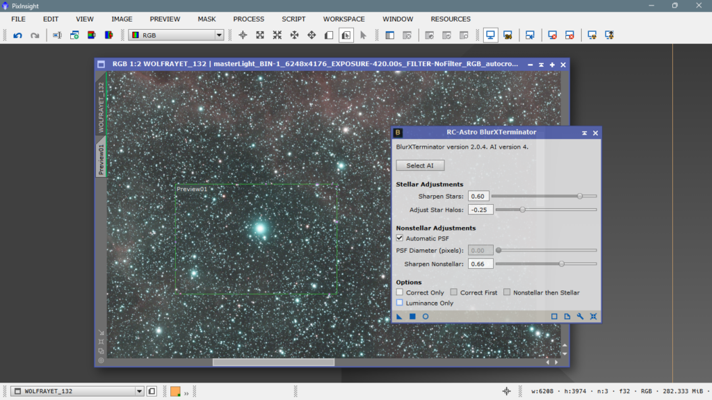
As we already have the shape well corrected, now we will correct the halos, the size and the punctuality of the stars, and to achieve this we will uncheck “Correct Only” and we will pay attention to the rest of the parameters to adapt them to our needs, each photo is different and will require some parameters or others.
The first thing we see in the photo is that the bright stars look fat and with a lot of halo, so we will make a preview to work faster and to be able to see immediately, what effect cause the parameters we have chosen.
As they are a little bit fat and with halo, in this case I have decided to increase the Sharpen Stars to 60 on a scale from 0 to 70, that is 85% more or less, this parameter will define the sharpness and diameter of the stars, I have also decided to increase the Adjust Star Halos in negative values to subtract brightness and give them a drier aspect, less unfocused, at the same time I have raised the Sharpen Nonstellar, that is, to focus non-stellar objects (nebulae) because let’s remember that if our stars are not punctual, the nebulae will not be either.
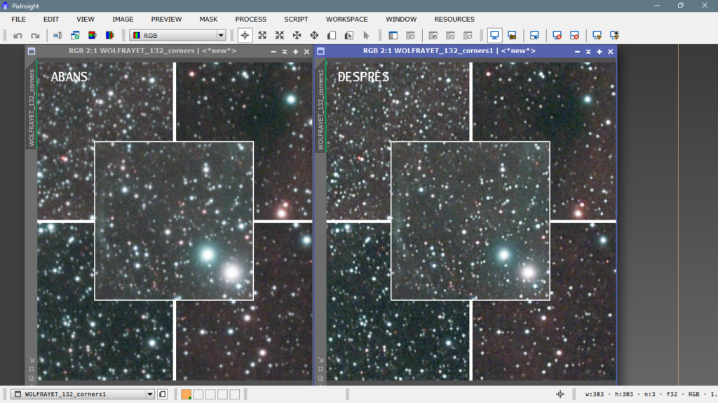
We apply it to the preview and see that the result looks really good, so we’ll go ahead and apply it to the whole image.
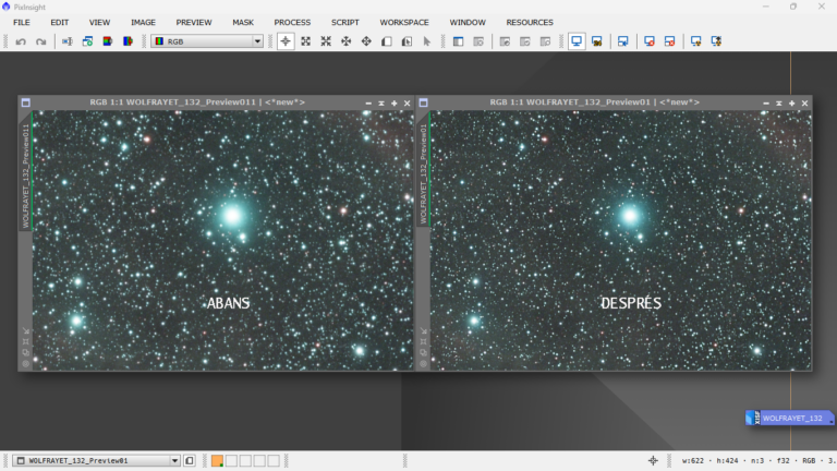
Getting this result.
The change is substantial, and now the logical next step is to correct the gradient—if there is one, of course. I’m doing it at this very moment for a very simple reason: a lot of people say that you should remove the noise before correcting gradients, but… how can I be sure that some of that so-called noise isn’t actually part of a real structure in the image? When working with such wide fields, you have to be really careful. I prefer to double-check and correct or confirm any potential gradients, because noise reduction could accidentally wipe out something that’s actually real.
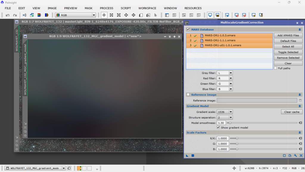
Alright, let’s move on to Multiscale Gradient Correction. In a previous article, I explained how to use it and what each parameter is for.
You can check out the article on MGC by clicking the following LINK.
It’s important to remember that before doing any of this, you need to calibrate the brightness of all the stars in the image using Spectrophotometric Flux Calibration. That workflow is also explained in the earlier article.
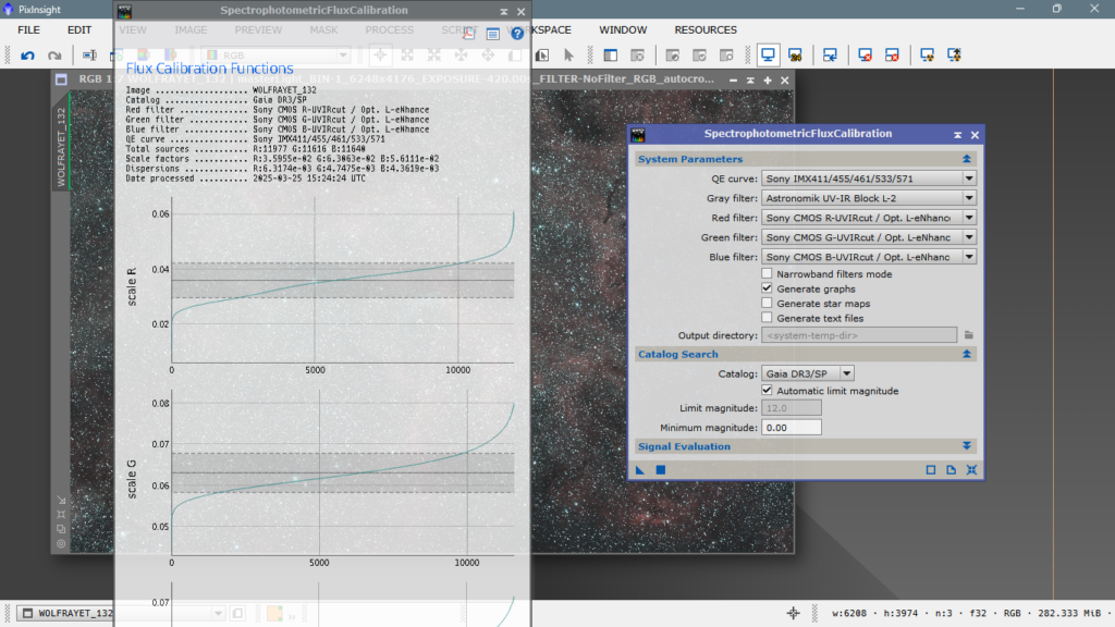
Once the stars’ flux has been calibrated and that information has been added to the image header, we move on with MGC and the correction of any potential gradients.
Since the image was taken under pretty good skies (Bortle 3) with no significant light pollution sources nearby, I decided to keep the correction fairly gentle.
Once we’ve corrected the gradient, the next logical step is to reduce small-scale or high-frequency noise. If we’ve got a good signal—meaning plenty of hours of exposure—this type of noise should be minimal, unless the object was captured very low on the horizon. That often happens with southern sky targets that have low declinations, for example, lower than DEC -10°.
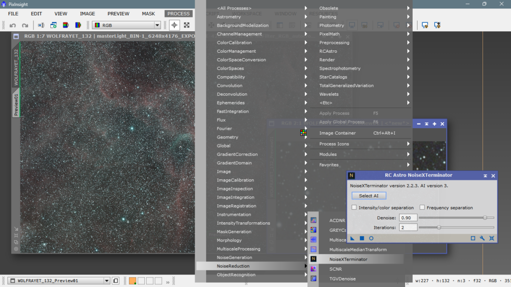
In my case, I use NoiseXterminator, but you can go with any noise reduction tool you prefer. I personally find this one to be the best by far—it lets me target the specific noise scale I want, and in this case, it’s the small-scale noise. You can also do this manually using A Trous Wavelets along with a mask, but this method is much faster and more effective.
That said, I’ll leave you a couple of links to some older videos I made years ago, where I walk through the manual process. You already know I’m a big fan of learning how to do things by myself before relying on third-party tools or scripts. Understanding the why and how behind each step is key.
Alright, let’s move on and identify the high-frequency noise, also known as small-scale or fine-grain noise.
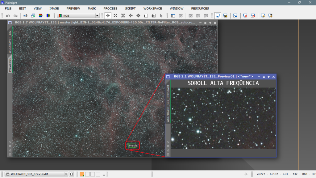
For now, I’m sticking with the default settings, since the image is quite solid in terms of total exposure time—almost 10 hours altogether. That gives us a pretty good signal-to-noise ratio, so there’s no urgent need to fine-tune the parameters just yet.
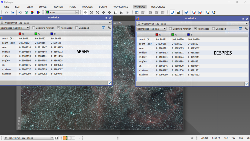
And once the noise reduction is applied, we’re left with a fantastic image—clean and free of noise. And remember, everything is still in the linear stage. Just take a look at the difference after cleaning it up—it’s pretty striking.
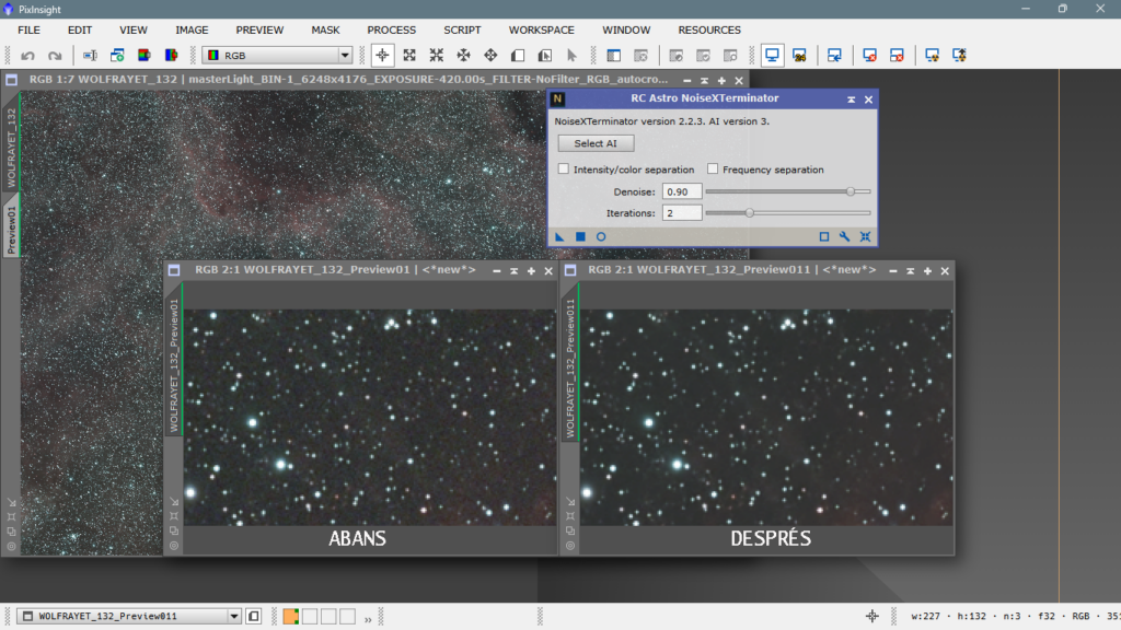
Even if we take a preview from a region with some nebula, we can clearly see how clean it looks—and how it hasn’t been blurred at all.
The next step is color calibration using Spectrophotometric Color Calibration. Here, we’ll tell it what sensor we used and which filters were involved, something like this:
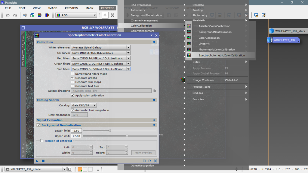
The calibration result:
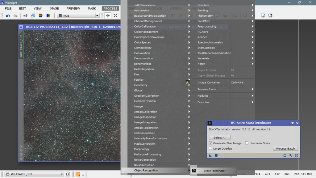
Well, let’s recap. We have a 10-hour image of WR-134 taken with a dual-band filter (Ha/OIII) from a good sky (Cinctorres refuge, Bortle 3). We’ve renamed it so we can easily manipulate the tabs. We’ve fixed the stars both morphologically and cosmetically, we’ve corrected possible gradients caused by the low light pollution at the capture site, we’ve removed high-frequency noise, also known as small-scale noise (down to 3/4 px), we’ve calibrated the color, and now, still in linear mode, we’ll extract the stars and separate them from the nebulae. We want to protect them. We don’t want to stretch them yet; we want to do it later, when all the nebulosity is already processed and illuminated, so we can more easily preserve its compact size and color. To do this, we’ll use the StarXterminator tool. You can also use Starnett++, but that’s the one I use.
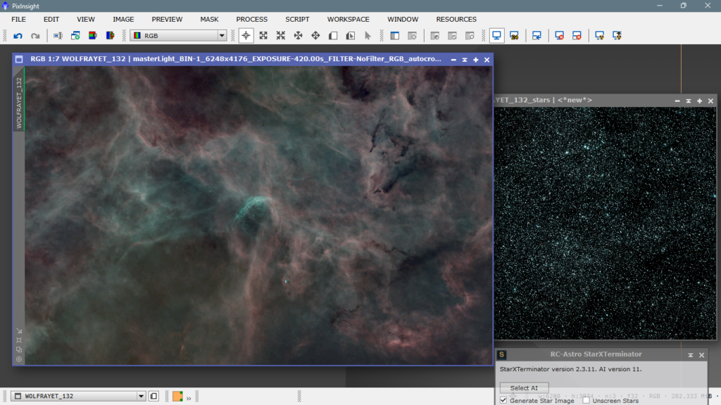
Simply, we will apply it as seen in the following image and the result will be an image with only stars and another, the original, with only nebulae.
Y el resultado:
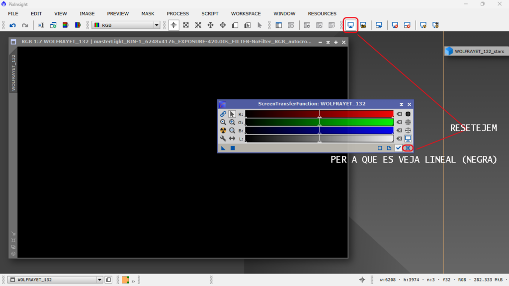
Once we have the stars separated from the nebula, we save them well, reset all the STF’s and start the real stretching with Masked Stretch, a native tool that stretches the image little by little and with each iteration it makes, it creates a mask to protect the brightest parts of the image, we can define how many iterations we want to do, the more iterations, the finer the thing will come out, it’s the way I like the most, there are many other ways to do it, but I use this one, I apply the default parameters, but first I reset so that when it’s finished being stretched we don’t see a false super saturated image.
We open Masked Stretch and apply the default values
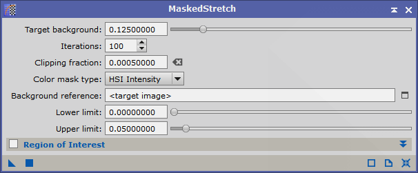
And this is the result:
We already have the image with the first one stretched, it seems dark, but it is an image that is saying process me now!! hehehe! For now we will not pay attention to the green, as it is a narrow band image made with a dual filter (Ha / OIII) and a color camera (RGGB) it turns out that for the green color there are two cells for each pixel, while for blue and red there is only one, it is the famous Bayer matrix, obviously the wave frequency corresponding to OIII is very close to green and blue, but closer to green, therefore, a lot of information has gone here, that is, 2 of green for every 1 of blue and one of red. If it had been a wideband image, for example, Pleiades, I would have paid attention and reduced the chrominance noise in the green channel with SCNR. However, with these narrowband images, I prefer to wait until the end and not literally erase information that could belong to OIII. This concept applies to any color cast in narrowband images.
In the next chapter, we’ll look at the rest of the NONLINEAR process: more stretching, more refocusing, color intensity, dynamic range modification—in other words, the entire process leading up to the final result.
See you next time!