How to Properly Use MGC to Fix Light Pollution in Your Photos
In this article, I’ll walk you through how to use the new Multiscale Gradient Correction tool to clean up light pollution gradients in your images.
The tool works by comparing your image against a massive, ever-growing astrophotometric database.
Basically, it builds a background model with the gradients, matching them against the MARS database, and using the astro and photometric data you’ve provided from your image.
This model is then used to correct the gradients without messing with the shape or brightness of the astronomical objects in your photo.
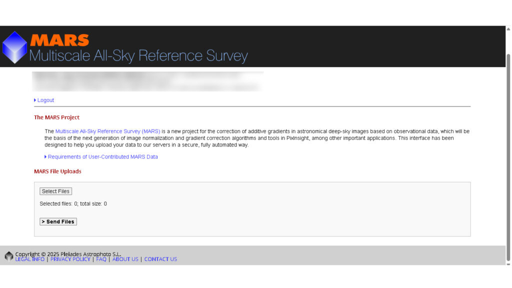
Of course, you’ll need to download the MARS catalogs first. Just head over to the downloads section on the Pléyades Astrophoto website and log in with your username and password.
Aquí tienes la traducción con el mismo tono informal, divulgativo y con el nivel técnico justo:
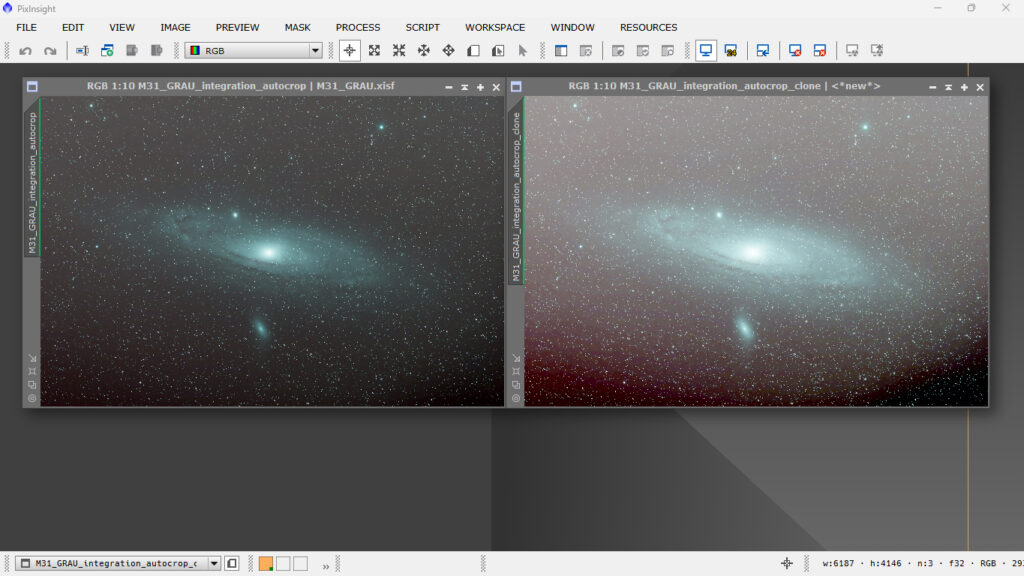
I picked an image of M31 taken from my apartment balcony — under pretty heavy light pollution. And what’s worse, there are tons of light sources around. One of the worst offenders (and kind of ironic) is the Planetarium of Castelló, which is super brightly lit and sits exactly to the east, right where my mount is pointed. Then there’s the Sant Pere football field, with those huge floodlight towers they use for training, the commercial port with its brightly lit customs area, and the port roundabout with this 25-meter-high pole topped with a ring of lights that honestly looks like a UFO. And that’s not even counting the street lights below and the ones right across from my place.
The image was taken with a 60mm refractor, a one-shot color (OSC) camera, and the well-known L-eNhance filter from Optolong. That filter is pretty much the only reason I can still get anything usable, stacking hour after hour of exposure time.
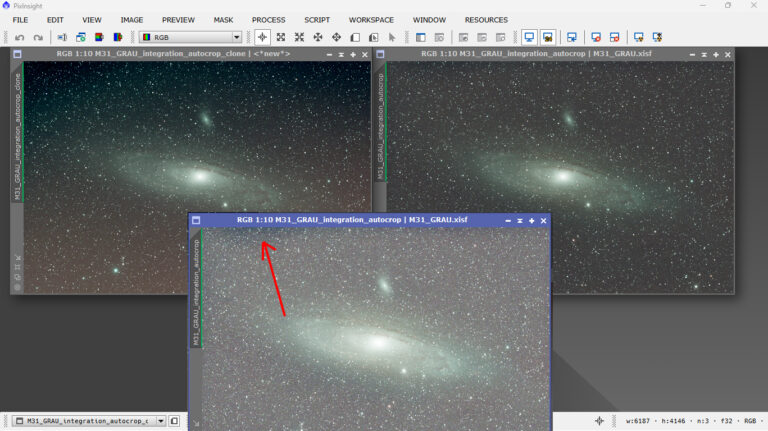
As you can see, the gradients are intense. I stretched the version on the right a bit more so you can better see just how bad the gradients really are.
Before reaching this step in the processing, I did some star repair using deconvolution (with BlurXT), and I also reduced a bit of noise with NoiseXT. It’s a good idea to do this early on — it helps the gradient correction tool work more effectively and produce better results.
It’s essential that the image has the astrometric solution embedded, so the program knows exactly where it is, what field you’re pointing at, and what object it is.
If you’re using cameras that write this info into the output files and you’re stacking with PixInsight, then you’re good to go — PixInsight picks it up automatically. But if you’re stacking with other software, you’ll need to provide that information manually.
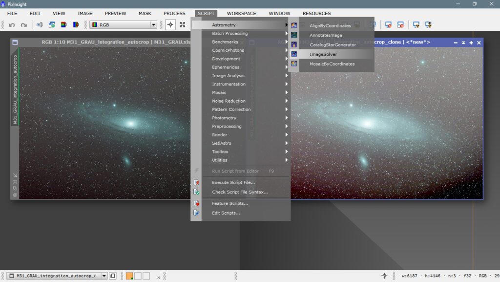
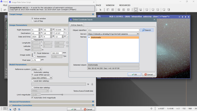
Just go to Script > Image Analysis > ImageSolver in PixInsight.
If you don’t know the exact coordinates, just click on “Search” and the program will look them up online. You only need to enter the name of the object, and it’ll automatically pull the right coordinates.
It’s super important to enter your pixel size and telescope focal length — this is how the tool knows what field of view to search for in your image. Without that info, it won’t be able to solve the image and will just fail to find anything.
It’s also a good idea to enter the capture date — at least the year — mainly because of stellar coordinate drift over time. PixInsight uses distortion models for its calculations, so this info helps it be more precise.
Once everything’s filled out properly, hit OK and move on with the processing.
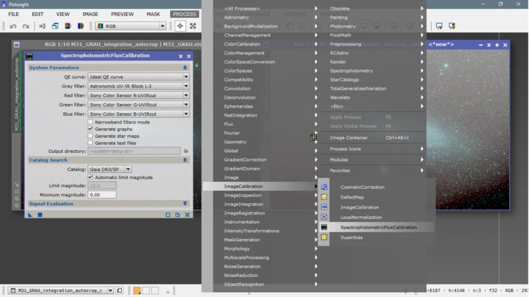
The next step is to calibrate the light profile of all the stars in your image using Spectrophotometric Flux Calibration. Since the program already knows which part of the sky and which object your image corresponds to, it simply compares your photo with existing catalogs and databases to see how far off your flux is — that is, how much your image deviates from the ideal light levels based on your camera, scope, and exposure time.
This process doesn’t make any visible changes to the image — it just adds essential metadata that allows you to keep working with more accurate and reliable data.
You can open this tool from ImageCalibration, Flux, or even from AllProcess.
Also, remember that to use these tools, you need to have the GAIADR3 and GAIADR3/SP astrometric catalogs downloaded and properly set up. These are available on the Peíades Astrophoto server.
You’ll need to download them to your PC, and then inside PixInsight, go to the GAIA section and set the correct path by clicking on the little wrench icon. [Link to the article on proper GAIA configuration]
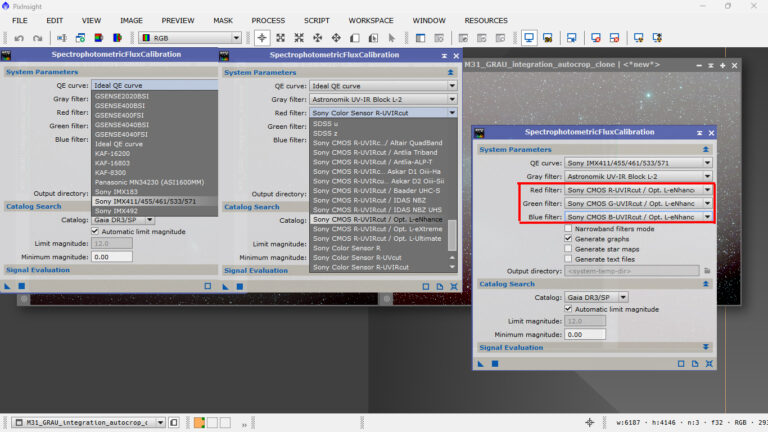
Now let’s set up the tool to calibrate the light flux of the stars in our image.
- Under Ideal QE curve, select your camera sensor. If it’s not listed, just leave the default setting.
- For Gray filter, leave it empty if you’re using a color camera.
- For Red filter, choose the option that most closely matches your setup. Browse through the menu — you’ll probably find something that fits, even if your exact camera and filter aren’t listed.
In my case, I used a Sony IMX571 sensor and an Optolong L-eNhance filter, so I selected those for each color channel.
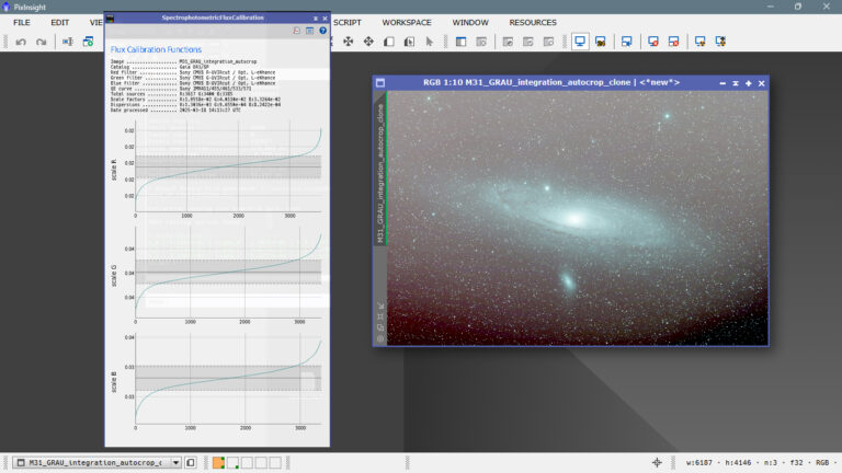
Once everything is properly set up, just hit the little square and apply — and that’s it! Your star field’s light flux profile is now calibrated and ready to go.
The graph shows, within the shaded area, which stars have been selected — basically, the ones used to build the illumination profile for the gradient model we’ll generate next with MGC.
Any parts of the graph that fall too low or spike too high might be due to variable stars, bad pixels, processing artifacts, or similar issues.
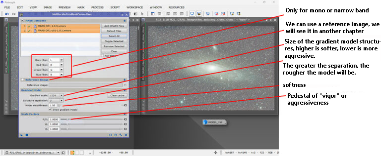
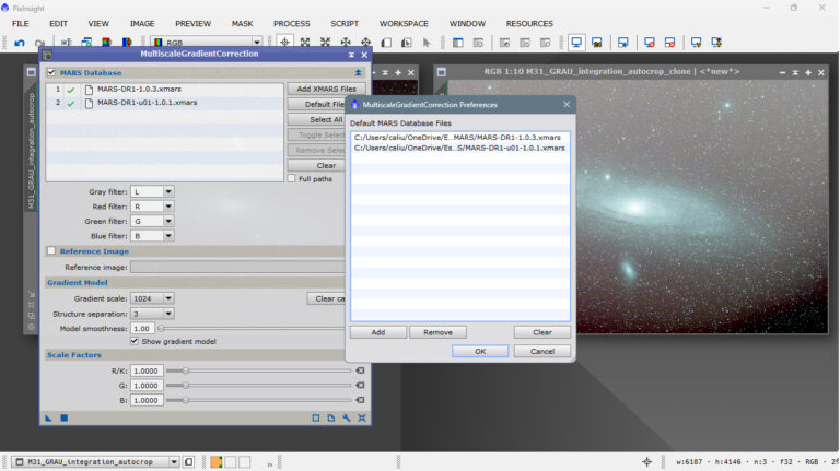
This is the dialog box for the MGC tool: Multiscale Gradient Correction.
To use it, we need to load the MARS files we downloaded from the *PixInsight website by clicking *Add/XMARS Files, or if you have it configured by default, click *Default Files.
I have it configured by default, and when I click *Default Files, the three catalogs are loaded automatically, so I don’t have to browse my computer every time looking for the files.
We’ve applied the default parameters and it worked very well, but the challenge is figuring out what each parameter is for and when and how to apply them. In theory, it’s «simple,» or rather, the theory is quite simple, but putting it into practice, not so much.
It involves creating a background model where only the gradients appear, a model where neither stars nor astronomical objects are present, so we can divide the model by the real image and get rid of the gradient, leaving us with an image with a very flat light profile.
This is physically impossible, but we can fine-tune it so that it appears to be so.
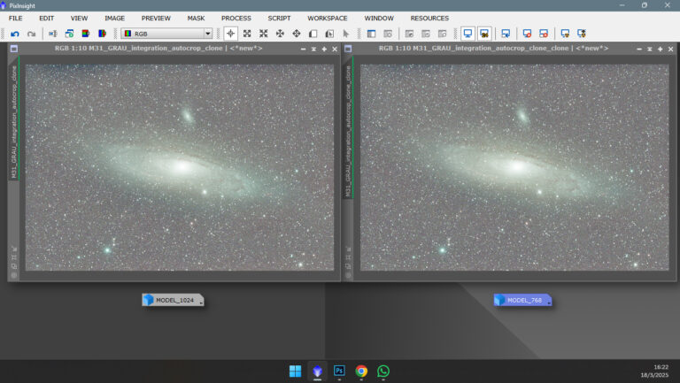
We need to investigate whether the gradients are large structures or, on the contrary, spots or very limited areas. In this specific case, the flats worked well, and we don’t have any spots or dark rings. Therefore, we can say that the gradients are large structures, and 1024 pixels, the default value, worked quite well. However, if we stretch the image further, we can still see traces of the gradient in the upper left corner.
We’ve lowered the GradientScale pixel dimension to 768 pixels, and it seems the gradient isn’t as evident anymore, although some remains. The logical thing to do would be to go down one more scale, but this is a double-edged sword. If you go down, you destroy the gradients, but you also destroy the details. So what happens? In photos taken against a low-quality sky with a lot of light pollution, the image won’t be very deep, and we won’t lose much. It wouldn’t be the same in a photo taken against a good sky and after a good handful of hours, a deep photo where we would subtract details from the background, which in that case would be disastrous.
Since it’s a very bright object and was taken at home, I can consider it fine, but first we’ll test what would have happened if we had continued downscaling, which is not advisable unless the photo is a mess of gradients, where we have no hope of getting a good one with a background full of details.
Below is an index of parameters.