Processing an image with everything against it: extremely low signal (30″), no darks, flats, or any calibration frames whatsoever, using a standard, unmodified, and uncooled DSLR camera—and to make matters worse, it’s a full-frame sensor.
In the following article, I’ll explain how I managed to obtain a decent image of the Rho Ophiuchi region using a camera with no astrophotography modifications. It’s a full-frame DSLR—specifically a stock Sony ILCE-7M III—and a 100 mm telephoto lens, the Tamron 70–180mm f/2.8 Di III VC VXD G2 @ f/2.8.
The 10-frame series at 30″ ISO 800 was taken by my friend Jose Del Valle Ruiz. You can check out his portfolio on Instagram—he has fantastic photos, both of astronomical landscapes and daytime photography. Definitely worth a visit.
I came across the image of the Rho Ophiuchi nebula complex on Facebook, and I was curious to see what could be extracted using PixInsight, being aggressive but without ruining the image. I say “aggressive” because if you don’t go bold, you’ll barely extract any information—30″ is very little signal.
The first thing I did was load the 10 files into WBPP for debayering, cosmetic correction, generating a local normalization reference, registering, stacking, and embedding the astrometric solution.
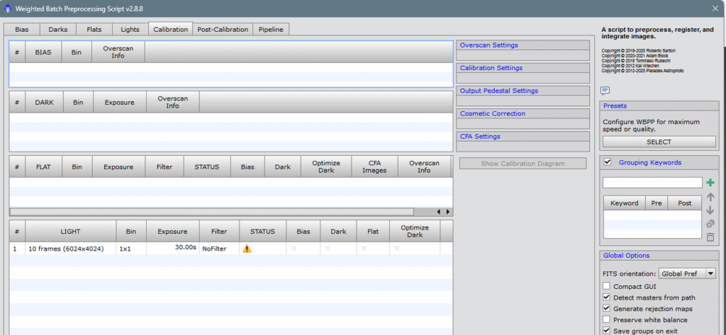
Then, I obtained the master file, i.e., the sum of the 10 individual frames (subframes). Let no one think that this «sum» equals 300″ of exposure (30×10=300)—it’s still just 30″ of exposure, but with less noise and a much better signal-to-noise ratio than a single frame. We’ll talk more about SNR in a future article—I’ll make a note of it.
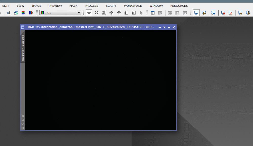
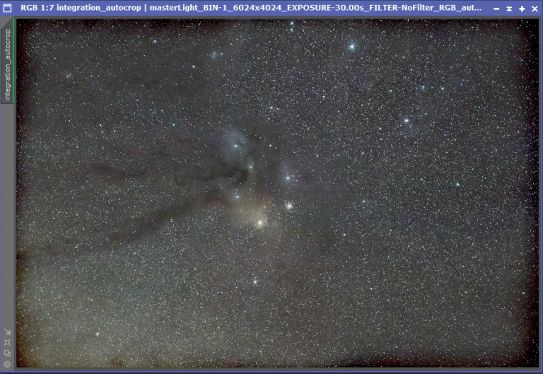
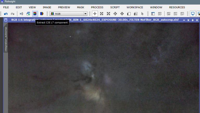
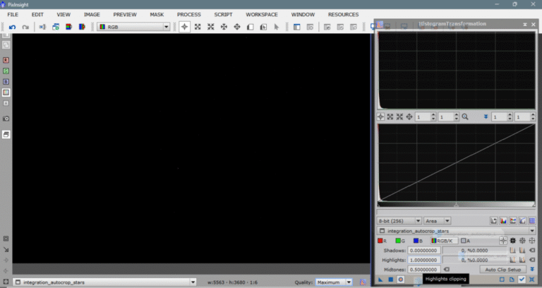
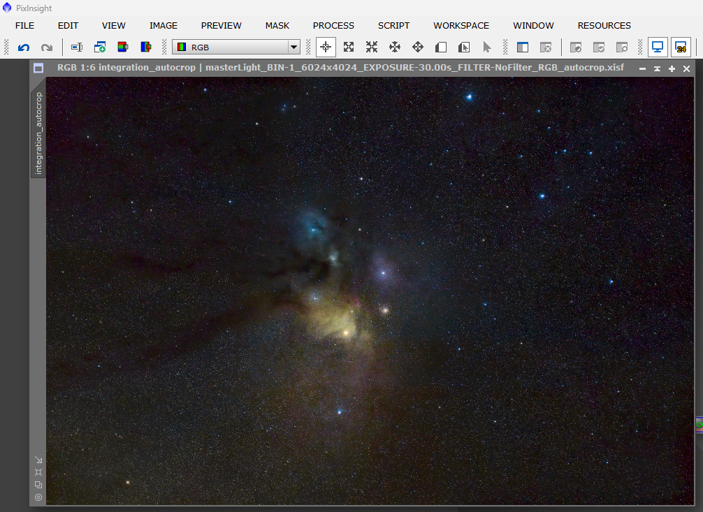
This is the linear file (unstretched):
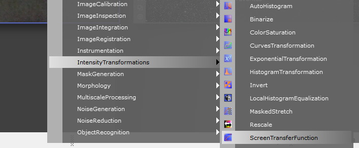
The first thing to do is apply STF (virtual stretch) to inspect the image and identify defects to correct. So, we click the “radioactive screen” icon while holding Ctrl to prevent all channels from being equally illuminated—this gives us a more comfortable virtual color calibration, rather than seeing everything green.
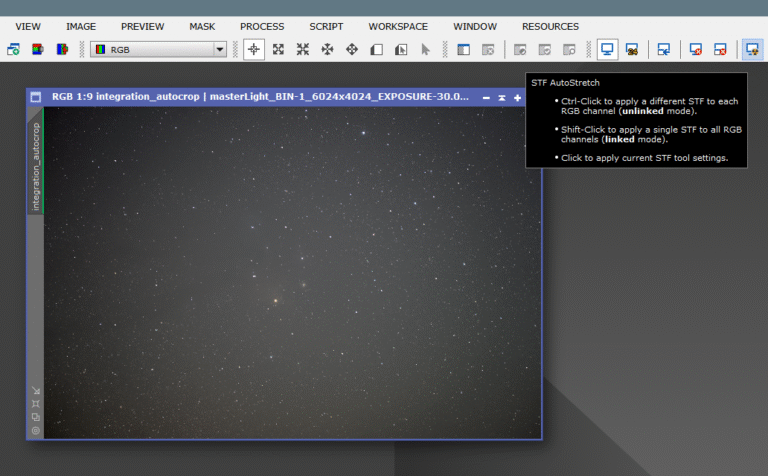
Keep in mind that the virtual stretch shown by STF is a “default” type, based on the program’s data analysis of the image. It’s the suggested result (so to speak). Of course, despite knowing we have very little signal, we always want to push further and extract the most from the photo—without ruining it visually.
First, we apply the workflow for linear images—analogously, “undeveloped.”
Since zooming in showed elongated corner stars, we’ll apply BlurXterminator in “Correct Only” mode (from RC-Astro, if we have it). If not, we can use a PixelMath operation that serves the same purpose. Here’s the LINK.
As you can see, the stars improved significantly—they’re now round. Previously, they were elongated due to lens distortion. With the script ImageAnalysis/AberrationSpotter, we can compare before and after applying BlurXterminator in Correct Only mode, which morphologically transforms the stars.
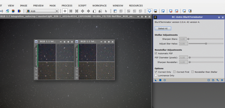
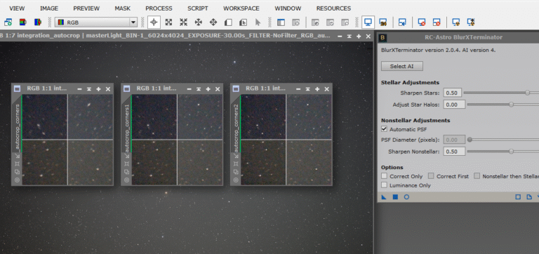
Next, we return to the same tool, but this time uncheck Correct Only to enable deconvolution and sharpening features—producing sharper, more defined stars and compensating for some defocus. The improvement is clear: from radial streaks to pinpoint stars. Look at the three previews at the image center—left to right shows the stars’ evolution after BlurXterminator.
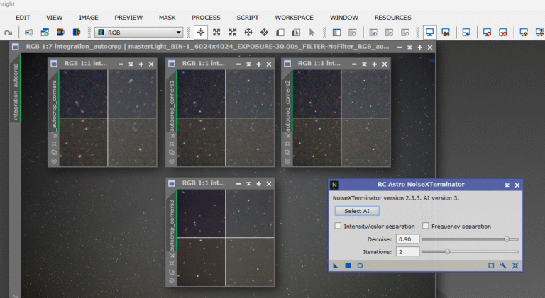
As is standard, after deconvolution, we apply noise reduction. I use NoiseXterminator, also from RC-Astro (Russell Croman), but any noise reduction tool will do.
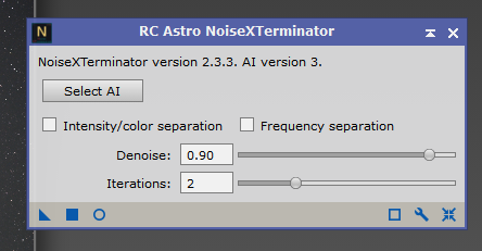
Compare the lower preview with the upper right one—you’ll see how, after noise reduction, stars appear sharper. It’s a visual effect—cleaning the background removes distractions and makes the image appear much clearer.
Next, we’ll calibrate the image’s light flow to improve gradient correction tools. The more metadata the tool has, the better. We do this with SPFC (SpectroPhotometric Flux Calibration).
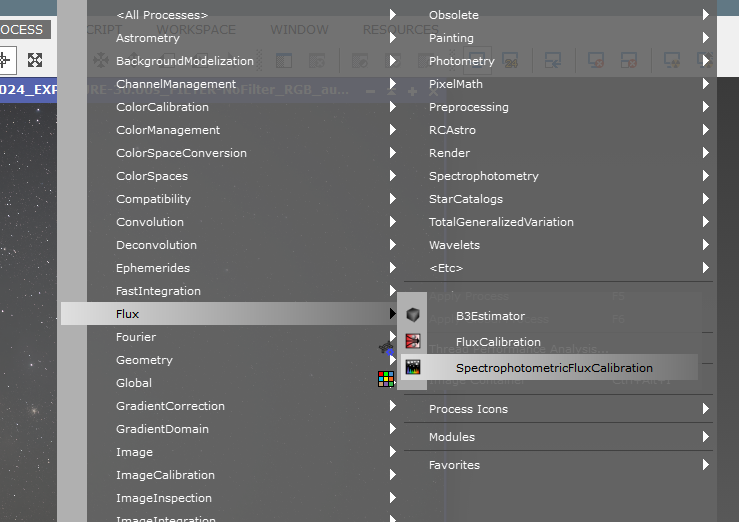
This tool doesn’t alter pixel values—it just adds metadata. Of course, you must configure it for your camera, sensor, and filters (if any).
Since the camera is a Sony with an Exmor (CMOS) sensor not listed in the calibration tool dropdown, we’ll input custom parameters:
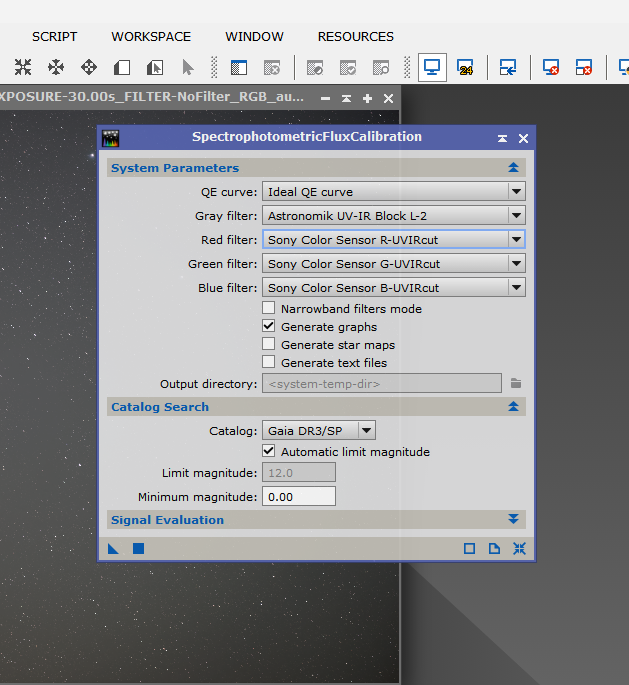
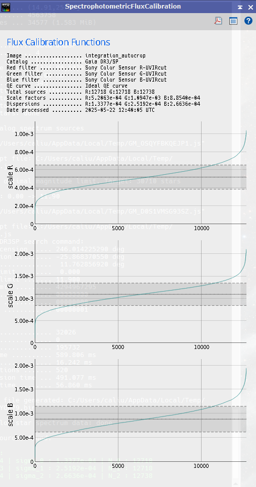
And obtain these light curves for each color channel:
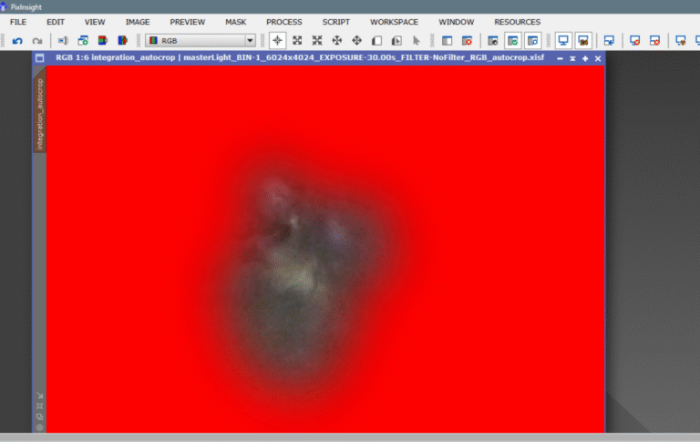
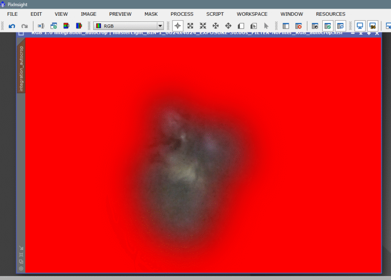
Now we proceed with gradient correction. The most prominent gradient is vignetting—caused by lens elements blocking uniform light across the sensor. This image lacks flats, darks, or bias frames, so the STF-stretched view clearly shows this defect.
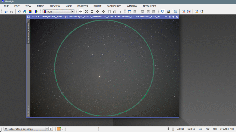
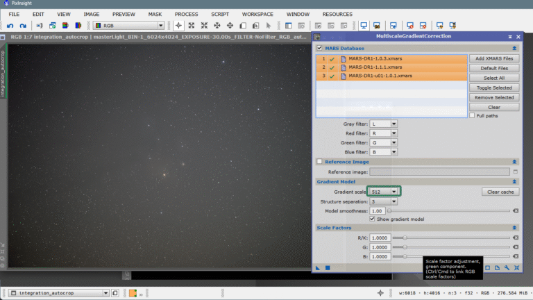
The farther from the center, the darker it gets. Since we couldn’t fix it during calibration, we’ll correct it now using MGC (Multiscale Gradient Correction)—a fantastic tool I discussed in a previous FOSC article. LINK
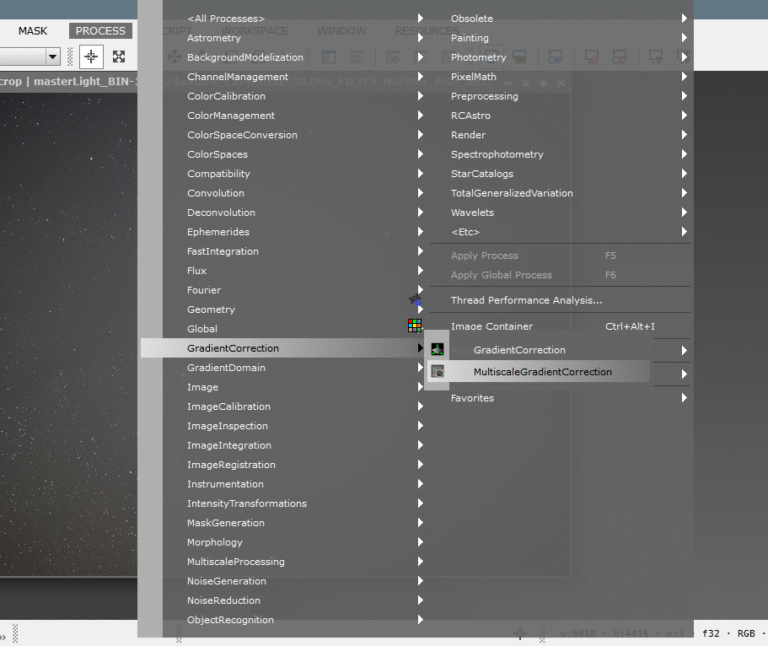
Because we don’t expect much from this image due to its low signal, we can afford to be aggressive with MGC—this is done by lowering the pixel size of structures in the background model, making it more defined and correcting vignetting more forcefully.
If you want to learn more about using MGC, how it works, and its settings, check out this LINK.
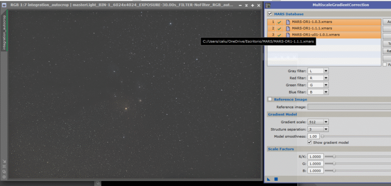
We open MGC, select all three available catalogs, and lower the scale to 512 px for stronger correction (in deeper, better images, we might use 1024 px or 2048 px).
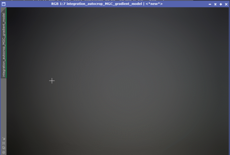
Once applied, the result is stunning.
Look at the gradient model MGC generated—it practically replaces the need for DBE or ABE. If not for dust and dirt, flats might not even be necessary. It’s a perfect flat. Look:
After enjoying this elegant and precise vignetting removal, we move on to color calibration—also explained in three languages and available in the FOSC index. LINK
Spectrophotometric Color Calibration (SPCC) uses quantum efficiency curves for various sensors and filters from its local database (customizable if you know how). You can create your own combinations based on your camera and filters. I explain this in another published article, available in the FOSC index in Valencian, Spanish, and English. LINK
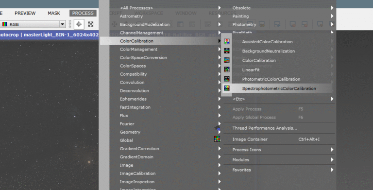
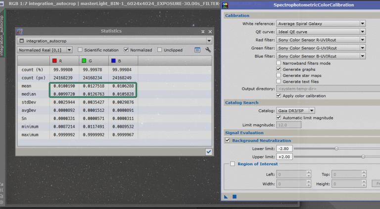
We must use the same parameters as with Flux calibration. Since the camera is unmodified and made for visible light, color calibration should be straightforward. We’ll open the statistics to compare before and after SPCC.
Before:
After:
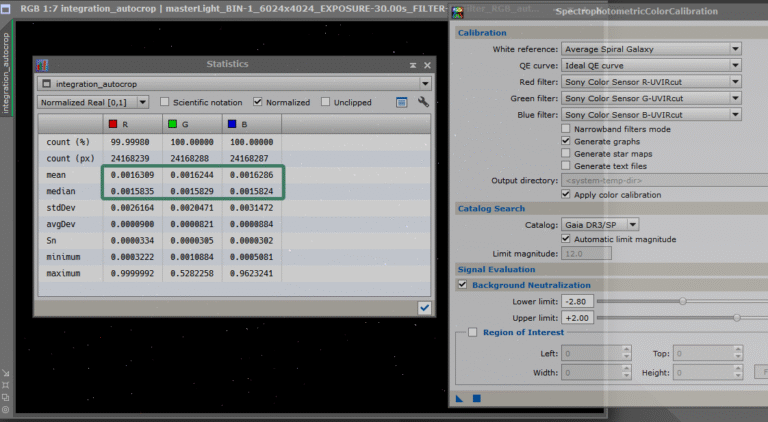
Perfectly balanced.
Next is the first stretch. Everyone has their preferred method. I personally like Masked Stretch—it gives results I like.
However, for this particular image (no calibration, very low signal), we’ll stretch it more conservatively using STF (Screen Transfer Function) as a guide for real stretch.
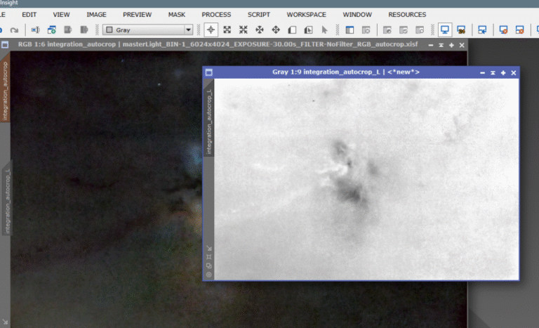
I also like separating stars before stretching. So, I’ll do that using StarXterminator (RC-Astro, of course).
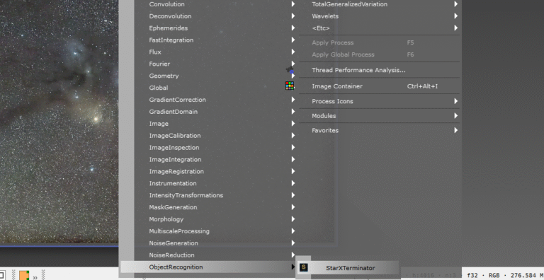
Open StarXterminator and check Generate Star Image to create a stars-only image for later reintegration.
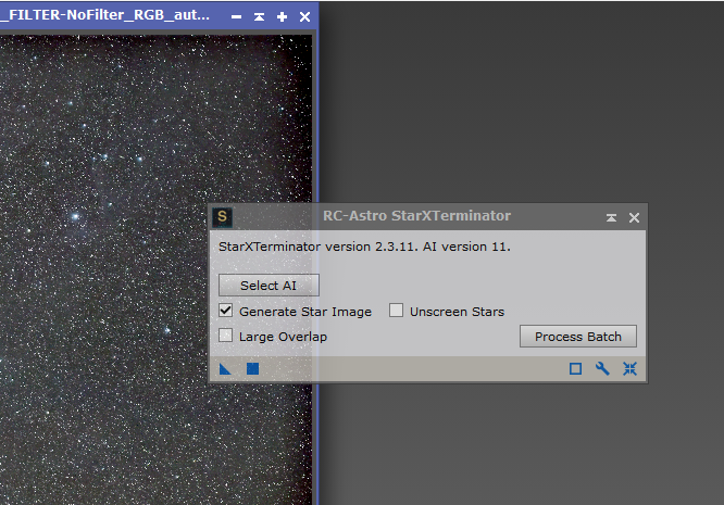
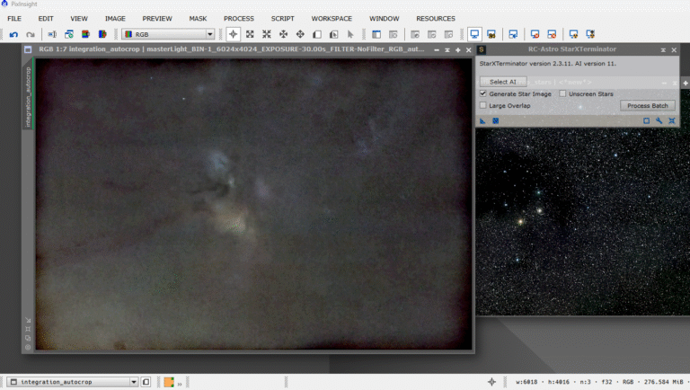
Once run, we get one image with nebulas only, and another with stars on a dark background.
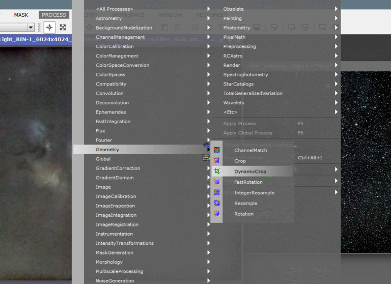
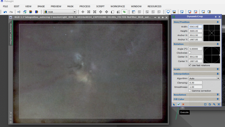
Next, we remove the black border—shadows from the sensor frame. Two ways: run aggressive MGC again at 128 px, or simply crop. But both images must be cropped identically. Here’s how using Dynamic Crop:
Click RESET
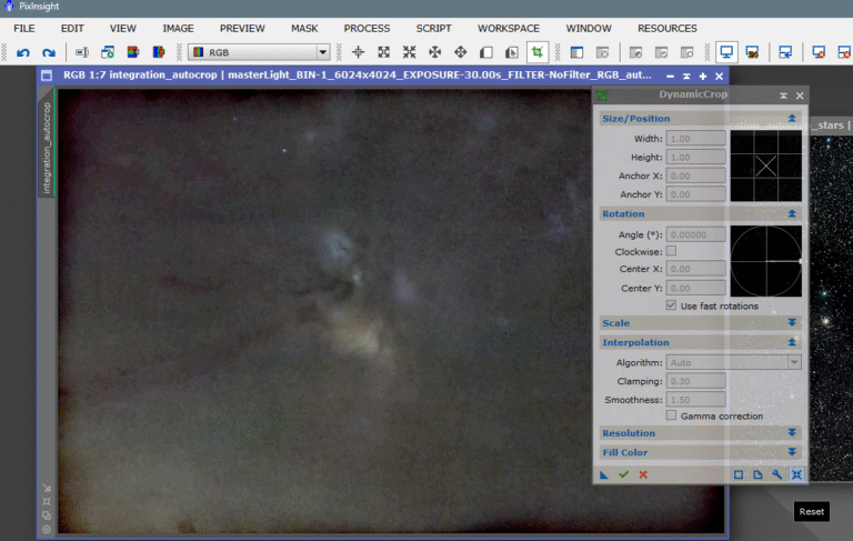
Select the area to keep
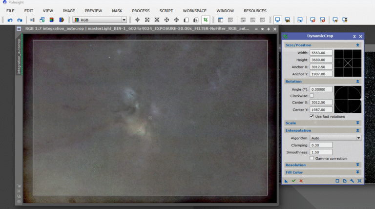
Drag the triangle onto the other image
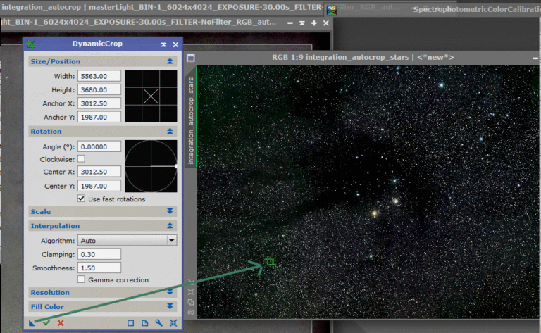
Click the green Execute stick
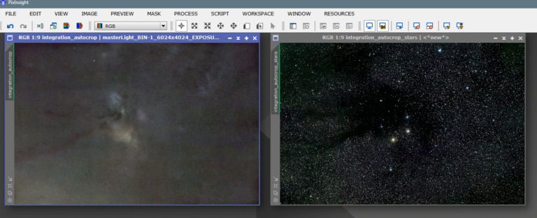
Now both images are identical in orientation and size—fully compatible.
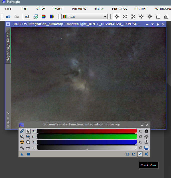
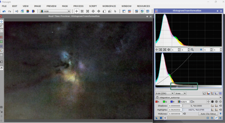
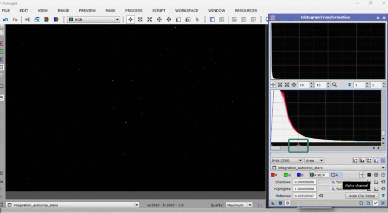
Alright, earlier we said we were going to stretch by making a «real» transfer from STF, which is a virtual view, to Histogram Transform, which is a real transformation—a NON-LINEAR transformation of the image. To do this, you need to open the STF console.
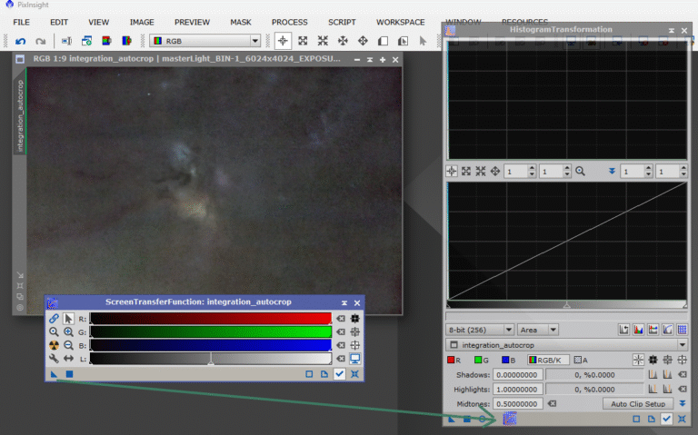
Next, with Track View enabled and the image we want to stretch also active (blue highlight), we will transfer those settings to the Histogram Transform console, simply by grabbing the triangle and dragging it to the bottom of the histogram window.
And now we drag and drop the triangle on the left onto the bottom part of the histogram window.
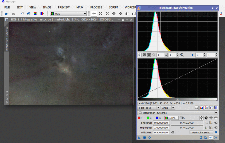
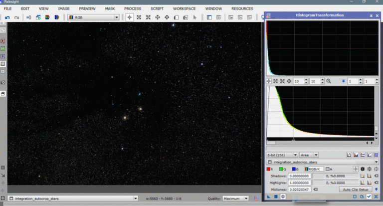
It’s important to say that the histogram must also have track view enabled and, once finished, everything must be reset to avoid having an overstretched view of the image. The result would be this:
Alright, we now have the image properly processed in LINEAR, we have stretched it, corrected the shape of the stars, reduced background noise, corrected vignetting and gradients, calibrated the color, separated the stars from the nebula, cropped the shadow from the sensor frame, and stretched only the photo of the nebulas—the stars will be stretched afterward. We do this to focus on processing the nebulosity without harming the stars.
The next thing our instincts tell us is to enhance the color and light of the little nebulosity we’ve captured, but at the same time, we don’t want to enhance the background; rather the opposite—the ideal would be to enhance all the nebulosity and darken the background, since it’s a nest of noise and imperfections caused by the low amount of signal.
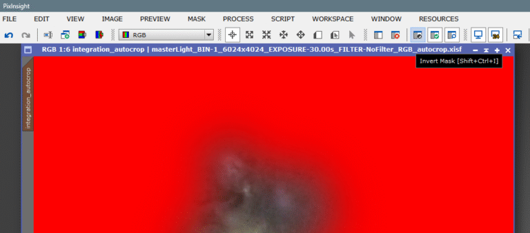
The idea is to make a mask that protects the nebulosity and exposes the background, which is almost useless, so that we can «turn it off» and focus on processing the other part. It’s difficult—clearly, there are dark structures that will be hard to discriminate in the mask and will be easy to darken by mistake—but we’ll try anyway.
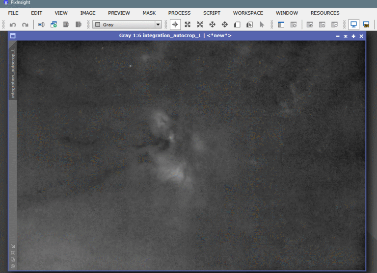
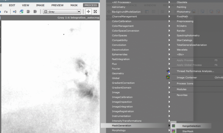
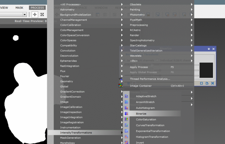
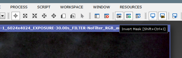
We will build the mask using the Range Mask tool, which is a very effective binarization tool because we can configure it to our liking; it has many parameters we can control. To make it easier, and before opening Range Mask, we will extract a luminance image in black and white and transform it with the histogram more softly to try to preserve the weaker structures. What we’ll do is invert it to better see the weaker nebular details.
We invert it (ctrl+I), open the histogram, and also enable real-time view (R-T).
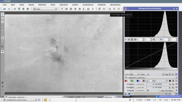
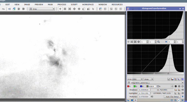
Now what we need to try is to get a white background, but at the same time visible structures—the more visible, the better. So we start moving the right arrow, the highlights arrow, to the left to brighten the background, to make it whiter—being careful not to erase the nebulas.
This might work.
We apply and move to Range Mask.
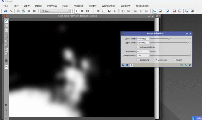
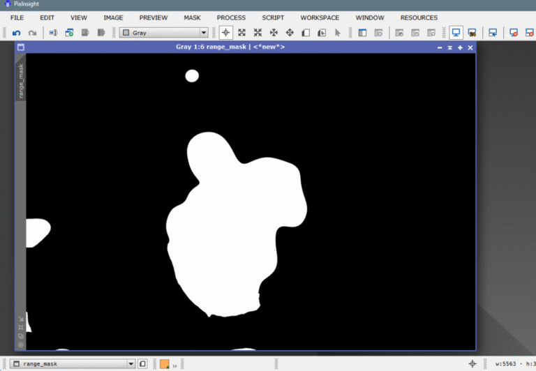
We open the console and activate the real-time view. I would leave it like this to start.
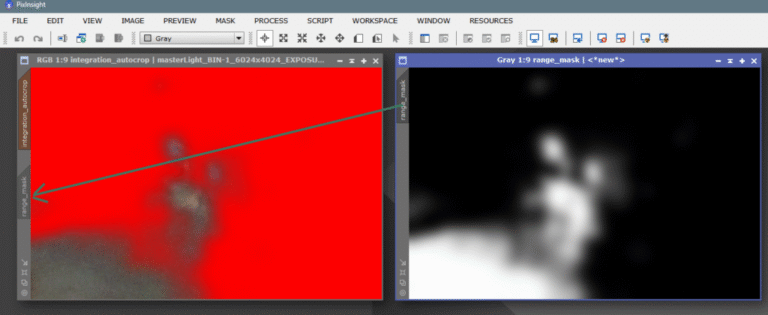
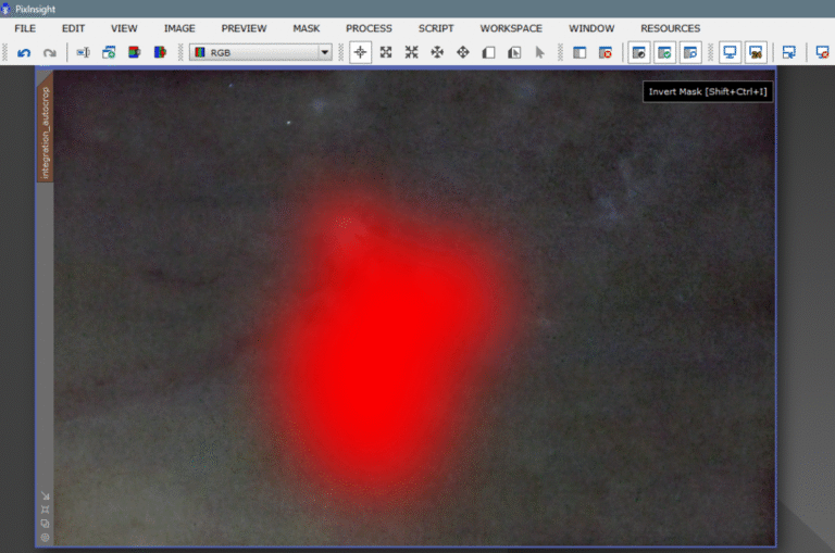
We apply and the mask is generated, but the problem is that the mask is imperfect—very imperfect—so we will overlay it on top of the main image to see what we need to erase and what not. We apply the mask over the main image simply by dragging the mask’s name tab to the side of the main image, below the name tab.
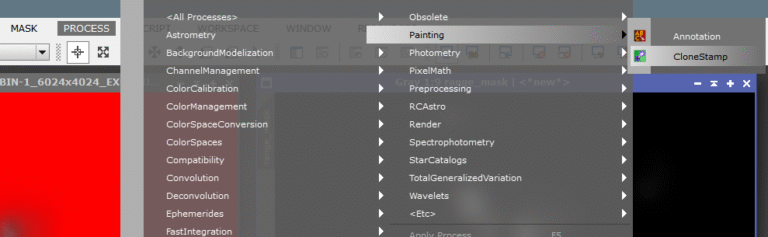
We can see there is an area at the bottom left that’s in the mask and is causing problems—we need to erase it. We’ll do it without deactivating the mask view and erasing directly over the other image, so we can see in real time what we’re doing. We open Clone Stamp from Painting and configure the tool.
We configure Clone Stamp—I’ve set the softness to maximum and chosen a size of 150, not too big nor too small. I’ve erased everything I didn’t like and applied it to the mask, which is still very imperfect. We want a rounder and more uniform shape, so we’ll go to the Binarize tool and give it some form.
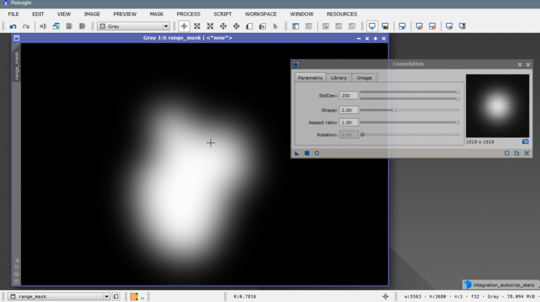
Now we need to smooth it and erase those white residues left scattered everywhere. We’ll erase again using Clone Stamp, and we’ll soften the result with the Convolution tool, which basically blurs images. We’ll increase it without fear, because if we leave the mask too harsh, later when processing with the mask applied, we’ll create artifacts on the mask edges and it’ll look pretty ugly.
The mask will look like this:
And now we’ll see how it performs over the main image.
That’s more like it, and it’s worth mentioning that if we wanted to perfect it even more, we’d just repeat the same process again and again, but for the purpose of illustrating this article, I think it’s enough.
Alright, now it’s time to decide what we’re going to process first—the background or the nebula. If we wanted to process the background first, we would have to invert the direction of the mask.
If we wanted to process the background first, we would need to invert the direction of the mask.
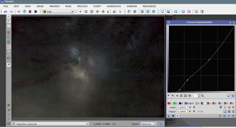
As we can see, the background has very subtle structures that we should try not to lose. Since it was impossible to make a mask to protect them, what we’ll do is proceed very carefully and take our time. We open the Curves and choose the light curve, the luminance channel, the L channel.
What I’m trying to do is darken the background while preserving as much as possible of these dark nebulas on the left that go straight to the Pipe Nebula, also known as LDN 1773.
It seems we’re slowly achieving it. Maybe I should transform the mask, but I’ll just avoid being too aggressive. Okay, we apply and then change the mask direction again by clicking the same icon as before.
Now the mask is inverted, protecting the background and exposing the nebulas. With ctrl+k (Show Mask), we can see it.
Now we go back to the curves and try to enhance what we have—the color in the C channel (chrominance) and the light of the different channels or the luminance channel (L). Remember that the C and L channels are antagonists—in other words, if we raise one, the other automatically drops. They are sworn enemies haha. I tried to add color with the C channel and light with the L channel. As you can see in the screenshot, I lowered the shadows of the L channel so that the mask edges wouldn’t be visible—an old dog’s trick haha.
Now, with a simple inverted luminance mask protecting it, we’ll make a slight histogram adjustment to bring it to life by raising the highlights and preparing it for the addition of the stars. No need to explain how to apply the mask again.
Now we open the histogram and raise the highlights a bit—just enough to bring it more to life, but not too much.
And now it’s time to add the stars. But remember—they’re not stretched yet. We’ll need to stretch them and give them a bit of color.
So let’s stretch and process the stars. First, we open the image we had minimized and also open the histogram window.
Before starting to stretch them, we have to consider one thing—in the «stars only» image, there aren’t just stars. There are also remnants of dark nebulosity that the algorithm couldn’t identify as nebula because they’re too dark and treated them as background. Our job will also be to try to show these nebulas without making the stars too big and saturated. It’s hard—but no one said this would be easy 😉
We’ll start by moving the midtones arrow (the middle one) halfway up the curve where the light begins to rise. We can zoom into the histogram using the mouse scroll.
Always with real-time view open to see what’s happening, we’ll apply it twice, and voilà—stretched stars and visible dust lanes.
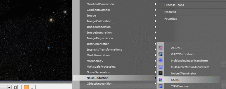
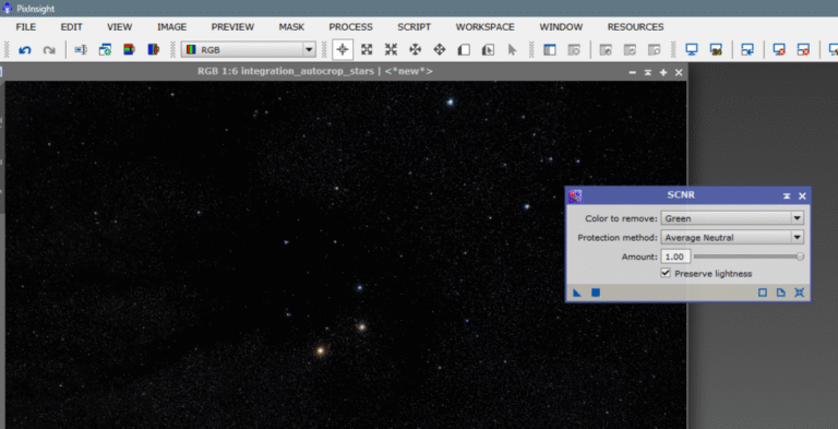
Now we just need to increase their color and add them to the main image, but there’s a detail we can’t overlook. We all know that green stars don’t exist—there’s no known green star (in the visible spectrum). So we’ll have to remove any trace of this color in the stars image. We’ll do this with the chromatic noise reduction tool called SCNR (Subtractive Chromatic Noise Reduction), using the default parameters for the green channel to remove any greenish hue.
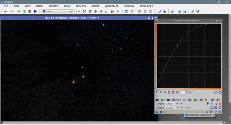
Once the excess green is removed from the stars, we’ll increase the quality and strength of the color by enhancing the chrominance channel or C channel from Curves. Always with Real-Time activated so we can see what’s happening, we raise the curve to taste and apply.
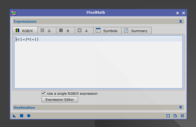
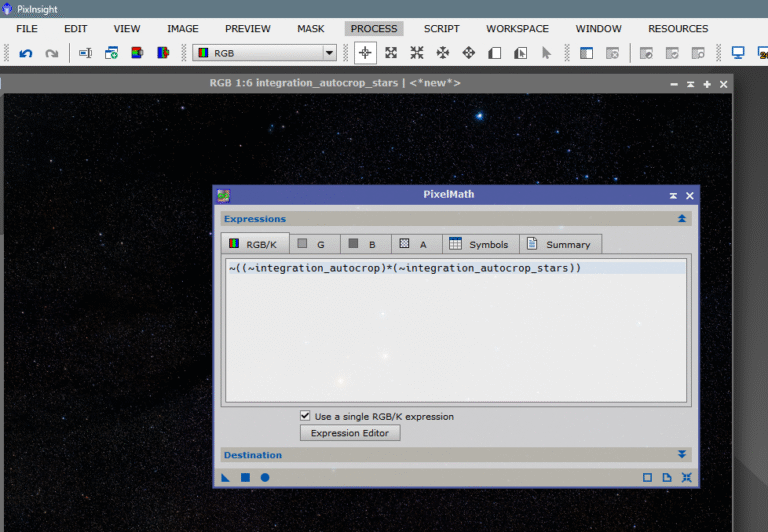
Once they’re how we want them, all that’s left is to recombine them with the main image. We’ll do this using a mathematical expression in Pixel Math—there are many, but this one is my favorite.
The result would look like this:
All that’s left is to apply.
Not bad for a 30″ image, right?
See you next time!